renv::restore()Open and reproducible analysis of light exposure and visual experience data (Beginner)
Preface
Wearables are increasingly used in research because they combine personalized, high‑temporal‑resolution measurements with outcomes related to well‑being and health. In sleep research, wrist‑worn actimetry is long established. As circadian factors gain prominence across disciplines, interest in personal light exposure has grown, spurring a variety of new devices, form factors, and sensor technologies. This trend also brings many researchers into settings where data from wearables must be ingested, processed, and analyzed. Beyond circadian science, measurements of light and optical radiation are central to UV‑related research and to questions of ocular health and development.
LightLogR is designed to facilitate the principled import, processing, and visualization of such wearable‑derived data. This document offers an accessible entry point to LightLogR via a self‑contained analysis script that you can modify to familiarize yourself with the package. Full documentation of LightLogR’s features is available on the documentation page, including numerous tutorials.
This document is intended for researchers with no prior experience using LightLogR, and assumes general familiarity with the R statistical software, ideally in a data‑science context1.
How this page works
This document contains the script for the online course series as a Quarto script, which can be executed on a local installation of R. Please ensure that all libraries are installed prior to running the script.
If you want to test LightLogR without installing R or the package, try the script version running webR, for a autonymous but slightly reduced version.
To run this script, we recommend cloning or downloading the GitHub repository (link to Zip-file) and running beginner.qmd. Alternatively, you can download the main script, the preview functions, and the data separately - though this is more laborious and error‑prone. In both cases, you’ll need to install the required packages. A quick way is to run:
Installation
LightLogR is hosted on CRAN, which means it can easily be installed from any R console through the following command:
install.packages("LightLogR")After installation, it becomes available for the current session by loading the package. We also require a number of packages. Most are automatically downloaded with LightLogR, but need to be loaded separately. Some might have to be installed separately on your local machine.
library(LightLogR) #load the package
library(tidyverse) #a package for tidy data science
library(gt) #a package for great tables
#the following packages are needed for preview functions:
library(cowplot)
library(legendry)
library(rnaturalearth)
library(rnaturalearthdata)
library(sf)
library(patchwork)
library(rlang)
library(glue)
library(gtExtras)
library(svglite)
library(downlit)
library(plotly)
library(webshot2)

#the next script will be integrated into the next release of LightLogR
#but have to be loaded separately for now (≤0.10.0)
source("scripts/overview_plot.R")

# Set a global theme for the background
theme_set(
    theme(
      panel.background = element_rect(fill = "white", color = NA)
    )
)
That is all we need to get started. Let’s make a quick visualization of a sample dataset that comes preloaded with the package. It contains six days of data from a participant, with concurrent measurements of environmental light exposure at the university rooftop. You can play with the arguments to see how it changes the output.
sample.data.environment |> #sample data
  gg_days(geom = "ribbon",
          aes_fill = Id,
          alpha = 0.6,
          facetting = FALSE
          ) |>
  gg_photoperiod(c(47.1, 9)) +
  coord_cartesian(expand = FALSE)
Import
File formats
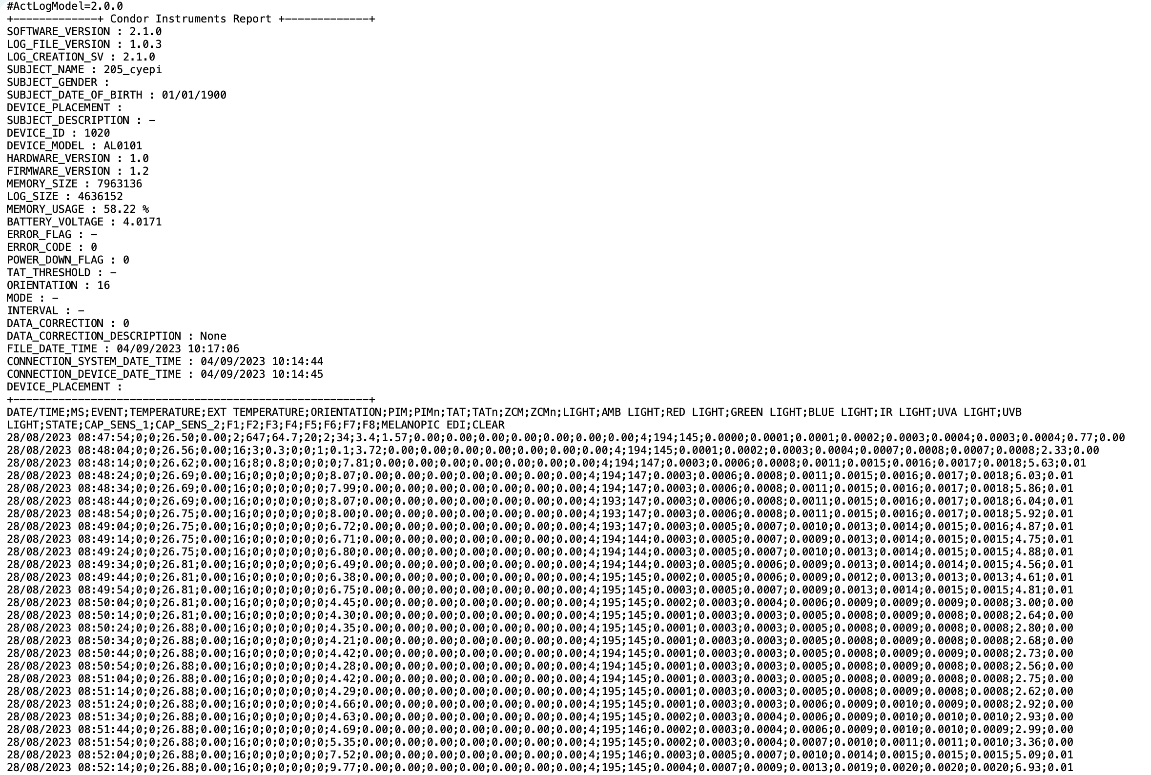
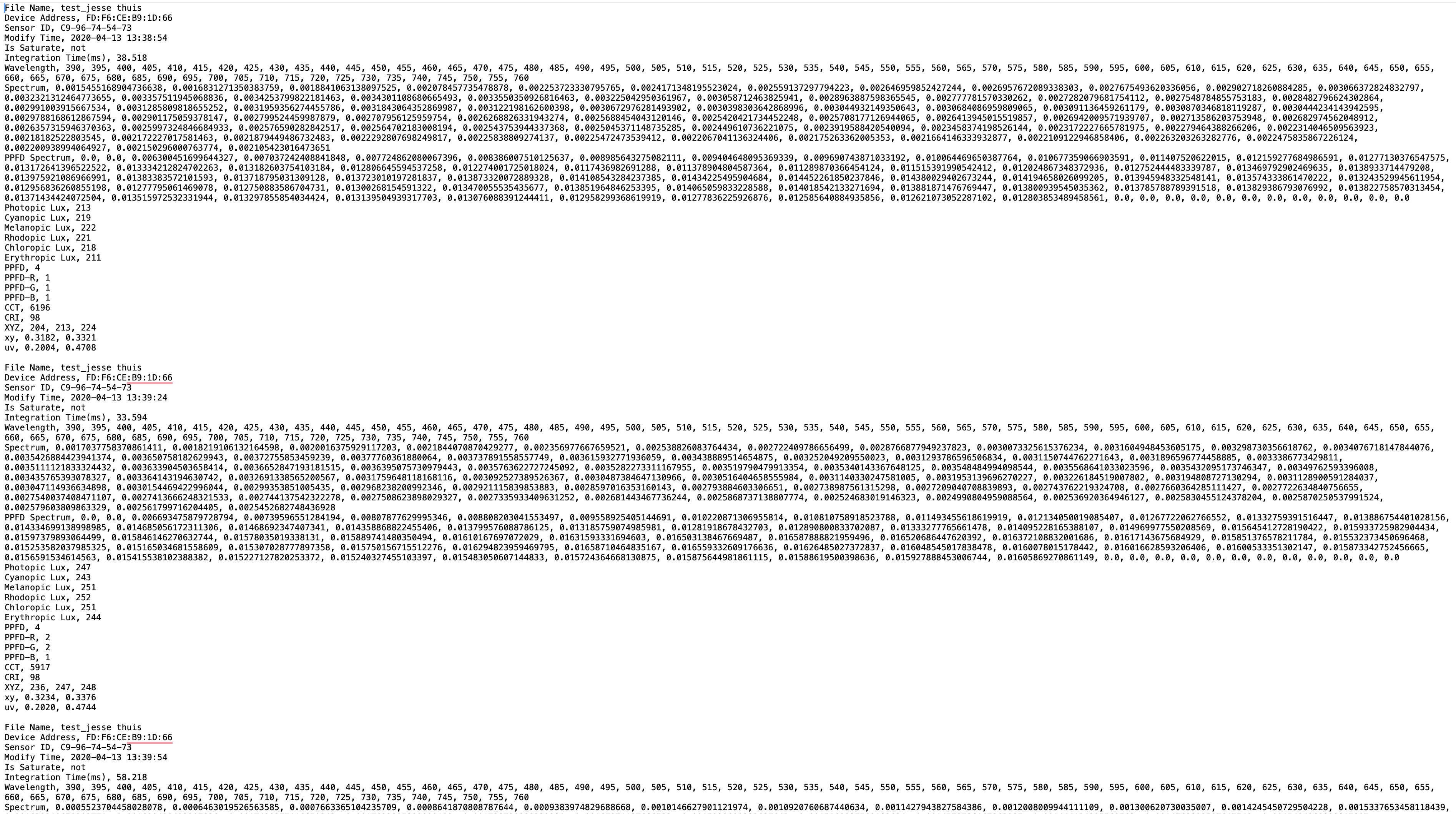
To work with LightLogR, we need some data from wearables. To the side are screenshots from three example formats to highlight the structure and differences. You can enlarge by clicking at them.
Importing a file
These files must be loaded into the active session in a tidy format—each variable in its own column and each observation in its own row. LightLogR’s device‑specific import functions take care of this transformation. Each function requires:
- filenames and paths to the wearable export files
- the time zone in which the data were collected
- (optional) participant identifiers
We begin with a dataset bundled with the package, recorded with the ActLumus device. The data were collected in Tübingen, Germany, so the correct time zone is Europe/Berlin.
#accessing the filepath of the package to reach the sample dataset:
filename <-
  system.file("extdata/205_actlumus_Log_1020_20230904101707532.txt.zip",
              package = "LightLogR")
dataset <- import$ActLumus(filename, tz = "Europe/Berlin", manual.id = "P1")Multiple files in zip: reading '205_actlumus_Log_1020_20230904101707532.txt'
Successfully read in 61'016 observations across 1 Ids from 1 ActLumus-file(s).
Timezone set is Europe/Berlin.

First Observation: 2023-08-28 08:47:54
Last Observation: 2023-09-04 10:17:04
Timespan: 7.1 days

Observation intervals:
  Id    interval.time     n pct
1 P1    10s           61015 100%
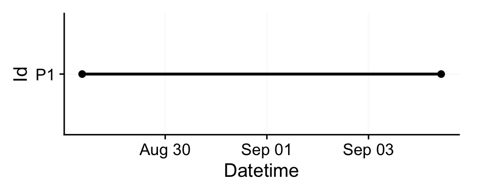
The import function also provides rich summary information about the dataset—such as the time span covered, sampling intervals, and an overview plot. Most import settings are configurable. To learn more, consult the function documentation online or via ?import. For a quick visual overview of the data across days, draw a timeline with gg_days().
dataset |> gg_days()We will go into much more detail about visualizations in the sections below.
Importing from a different device
Each device exports data in its own format, necessitating device‑specific handling. LightLogR includes import wrapper functions for many devices. You can retrieve the list supported by your installed version with the following function:
 [1] "Actiwatch_Spectrum" "ActLumus"           "ActTrust"
 [4] "Circadian_Eye"      "Clouclip"           "DeLux"
 [7] "GENEActiv_GGIR"     "Kronowise"          "LiDo"
[10] "LightWatcher"       "LIMO"               "LYS"
[13] "MiEye"              "MotionWatch8"       "nanoLambda"
[16] "OcuWEAR"            "Speccy"             "SpectraWear"
[19] "VEET"
We will now import from two other devices to showcase the differences.
Speccy
filename <- "data/beginner/Speccy.csv"
dataset <- import$Speccy(filename, tz = "Europe/Berlin", manual.id = "P1")
Successfully read in 1'336 observations across 1 Ids from 1 Speccy-file(s).
Timezone set is Europe/Berlin.

First Observation: 2023-08-31 09:34:26
Last Observation: 2023-09-01 07:49:26
Timespan: 22 hours

Observation intervals:
  Id    interval.time        n pct
1 P1    60s (~1 minutes)  1335 100%
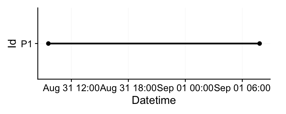
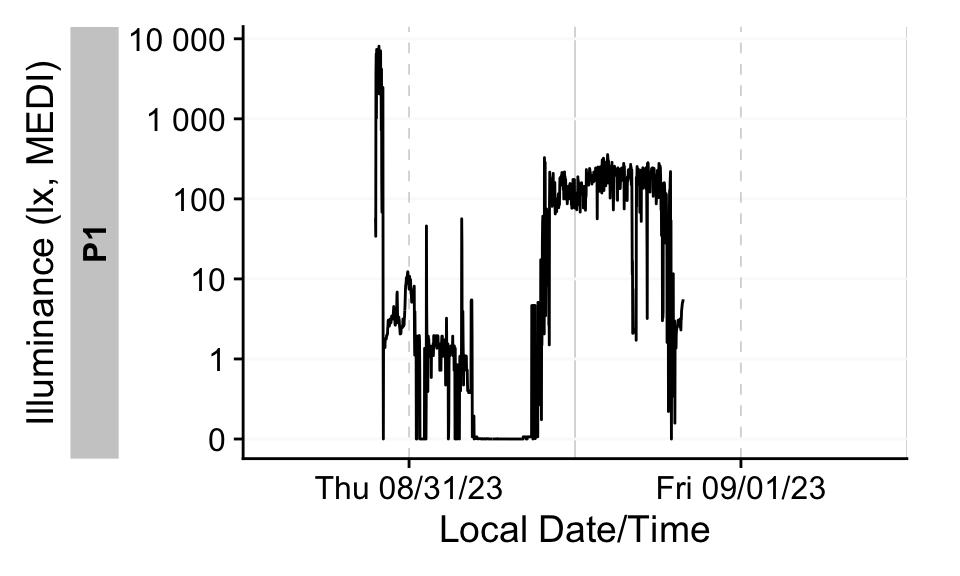
dataset |> gg_days()nanoLambda
filename <- "data/beginner/nanoLambda.csv"
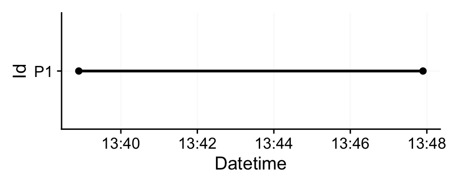
dataset <- import$nanoLambda(filename, tz = "Europe/Berlin", manual.id = "P1")
Successfully read in 19 observations across 1 Ids from 1 nanoLambda-file(s).
Timezone set is Europe/Berlin.

First Observation: 2020-04-13 13:38:54
Last Observation: 2020-04-13 13:47:54
Timespan: 9 mins

Observation intervals:
  Id    interval.time     n pct
1 P1    30s              18 100%
If we try to visualize this dataset as we have done above, we get an error.
dataset |> gg_day()This is because many LightLogR functions default to the melanopic EDI variable2. However, the nanoLambda export does not include this variable. Therefore, we must explicitly specify which variable to display. Let’s inspect the available variables:
dataset |> names() [1] "Id" "File_Name" "Device_Address"
[4] "Sensor_ID" "Datetime" "Is_Saturate"
[7] "Integration_Time(ms)" "Wavelength" "Spectrum"
[10] "PPFD_Spectrum" "Photopic_Lux" "Cyanopic_Lux"
[13] "Melanopic_Lux" "Rhodopic_Lux" "Chloropic_Lux"
[16] "Erythropic_Lux" "PPFD" "PPFD-R"
[19] "PPFD-G" "PPFD-B" "CCT"
[22] "CRI" "XYZ" "xy"
[25] "uv" "file.name" You can choose any numeric variable; here, we’ll use Melanopic_Lux, which is similar—though not identical—to melanopic EDI. To identify which argument to adjust, consult the function documentation:
?gg_day()Use the y.axis argument to select the variable. Also update the axis title via y.axis.label; otherwise the default label will refer to melanopic EDI.
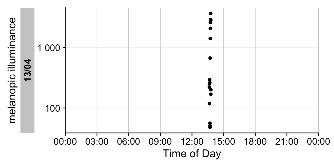
Because this dataset spans only a short interval of about 9 minutes, we’ll visualize it with gg_day(), which uses clock time on the x‑axis. There are a few other differences to gg_days(), which we will see in the sections below.
dataset |> gg_day(y.axis = Melanopic_Lux, y.axis.label = "melanopic illuminance")In summary, importing from different devices is typically as simple as specifying the device name. Some devices require additional arguments; consult the ?import help for details.
Importing more than one file
In typical studies, you’ll work with multiple participants, and importing each file individually is cumbersome. LightLogR supports batch imports; simply pass multiple files to the import function. In this tutorial, we’ll use three files from three participants, all drawn from the open‑access personal light‑exposure dataset by Guidolin et al. 20253. All data were collected with the ActLumus device type.
When importing multiple files, keep the following in mind:
- All files must originate from the same device type, share the same export structure, and use the same time‑zone specification. If they differ, import them separately.
- Be deliberate about participant‑ID assignment. The
manual.idargument used above would assign the same ID to all imported data in a batch. If a file contains a column specifying theId, you can point to that column; more often, the identifier is encoded in the filename. If you omit ID arguments, the filename is used asIdby default. Because filenames are often verbose, you will typically extract only the participant code. In our three example files, the relevant IDs are216,218, and219.
filenames <- list.files("data/beginner", pattern = "actlumus", full.names = TRUE)
filenames
[1] "data/beginner/216_actlumus_Log_1382_20231009130709885.txt"
[2] "data/beginner/218_actlumus_Log_1020_2023102309585329.txt"
[3] "data/beginner/219_actlumus_Log_1382_20231023113046652.txt"If filenames follow a consistent pattern, you can instruct the import function to extract only the participant code from each name. In our case, the first three digits encode the ID. We can specify this with a regular expression: ^(\d{3}). This pattern matches the first three digits at the start of the filename and captures them (^ = start of string, \d = digit, {3} = exactly three, (& ) = encloses the part of the pattern we actually want). If you’re not familiar with regular expressions, they can look like a jumble of ASCII characters, but they succinctly express patterns. Large language models are quite good at proposing regexes and explaining their components, so consider prompting one when you need a new pattern. With that, we can import our files.
pattern <- "^(\\d{3})"
dataset <- import$ActLumus(filenames, tz = "Europe/Berlin", auto.id = pattern)
Successfully read in 184'333 observations across 3 Ids from 3 ActLumus-file(s).
Timezone set is Europe/Berlin.

First Observation: 2023-09-29 14:40:52
Last Observation: 2023-10-23 11:29:10
Timespan: 24 days

Observation intervals:
   Id    interval.time            n pct
 1 216   10s                  61760 100%
 2 216   19s                      1 0%
 3 216   240718s (~2.79 days)     1 0%
 4 218   8s                       1 0%
 5 218   10s                  60929 100%
 6 218   11s                      1 0%
 7 219   9s                       1 0%
 8 219   10s                  61634 100%
 9 219   16s                      1 0%
10 219   583386s (~6.75 days)     1 0%
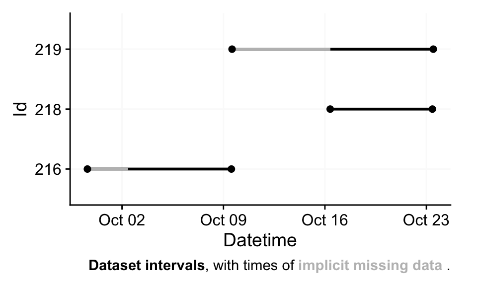
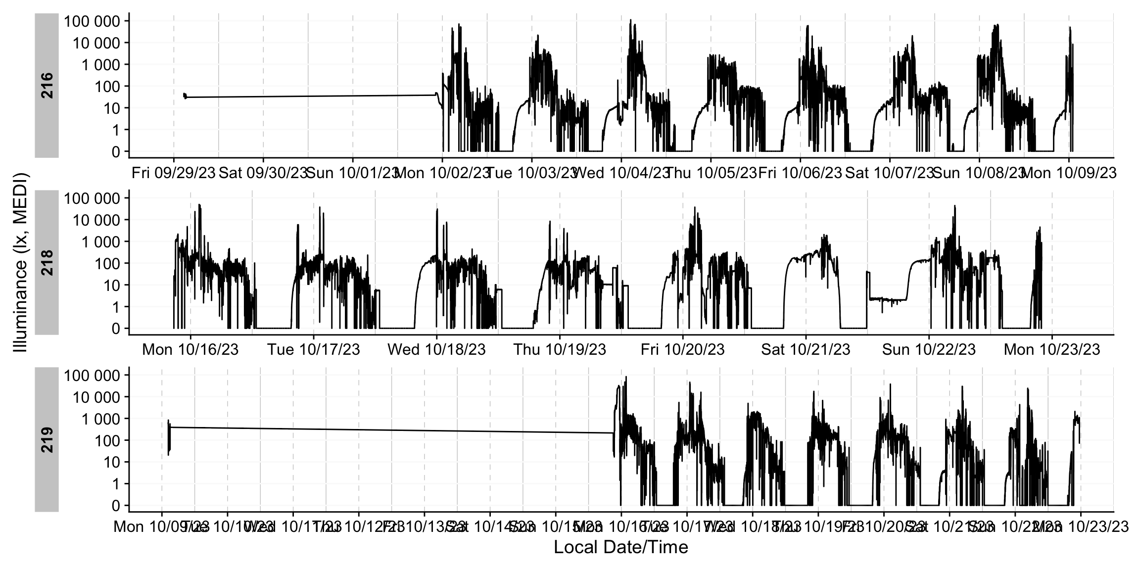
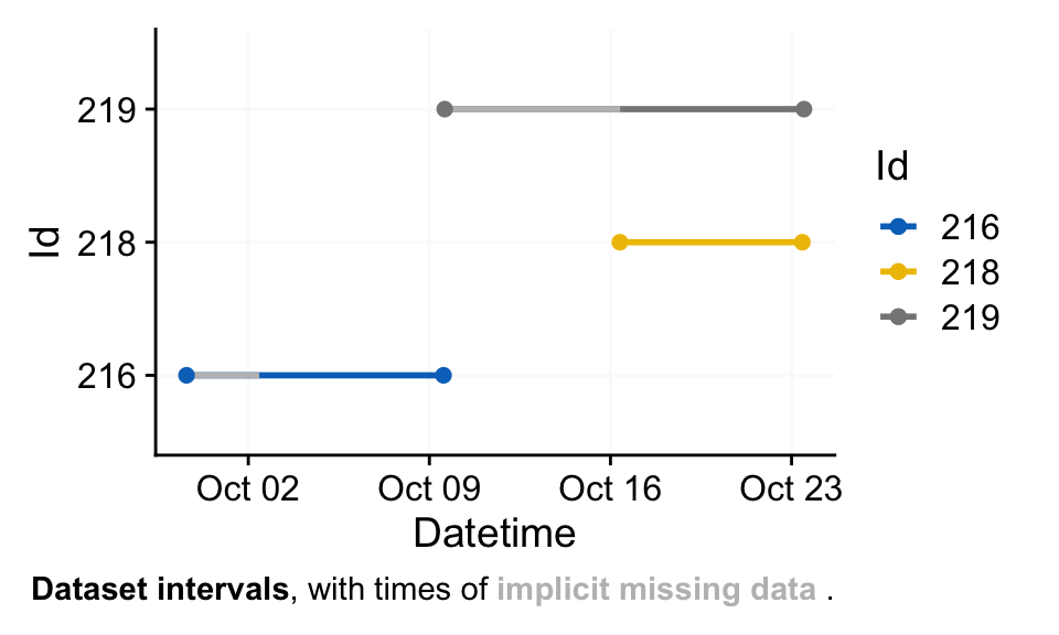
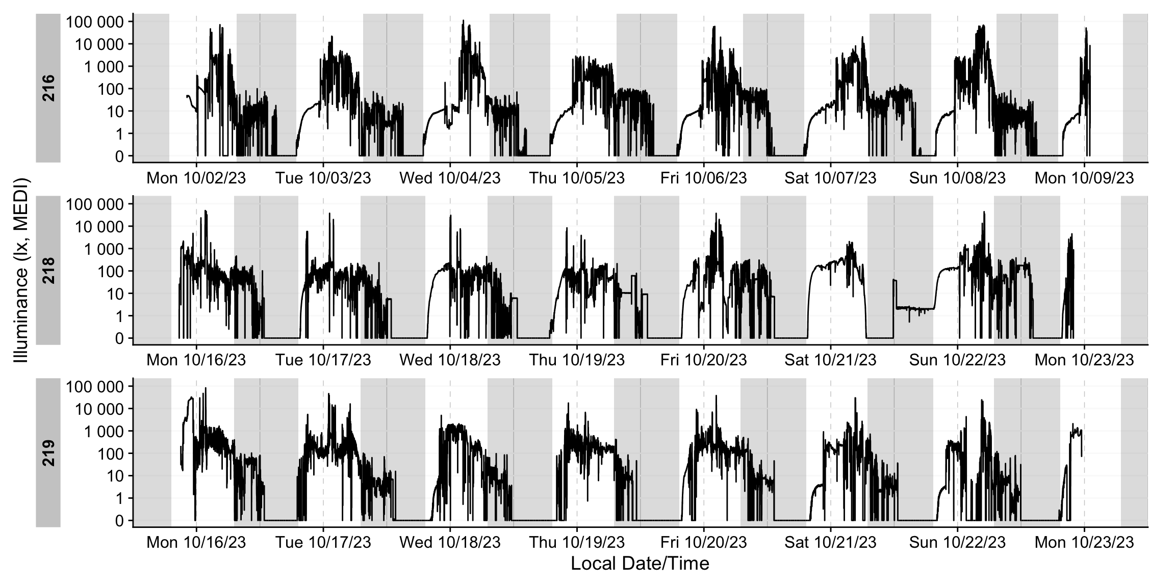
The overview plot is now more informative: it shows how the datasets align across time and highlights extended gaps due to missing data. We will return to the terminology of implicit missingness shortly.
dataset |> gg_days()Direct plotting highlights the extended gaps in the recordings. We’ll apply a package function that removes days with insufficient coverage to address this. For now, we can ignore the details: any participant‑day with more than 80% missing data will be excluded.
dataset_red <-
  dataset |>
  remove_partial_data(
    Variable.colname = MEDI,
    threshold.missing = 0.8,
    by.date = TRUE,
    handle.gaps = TRUE
  )

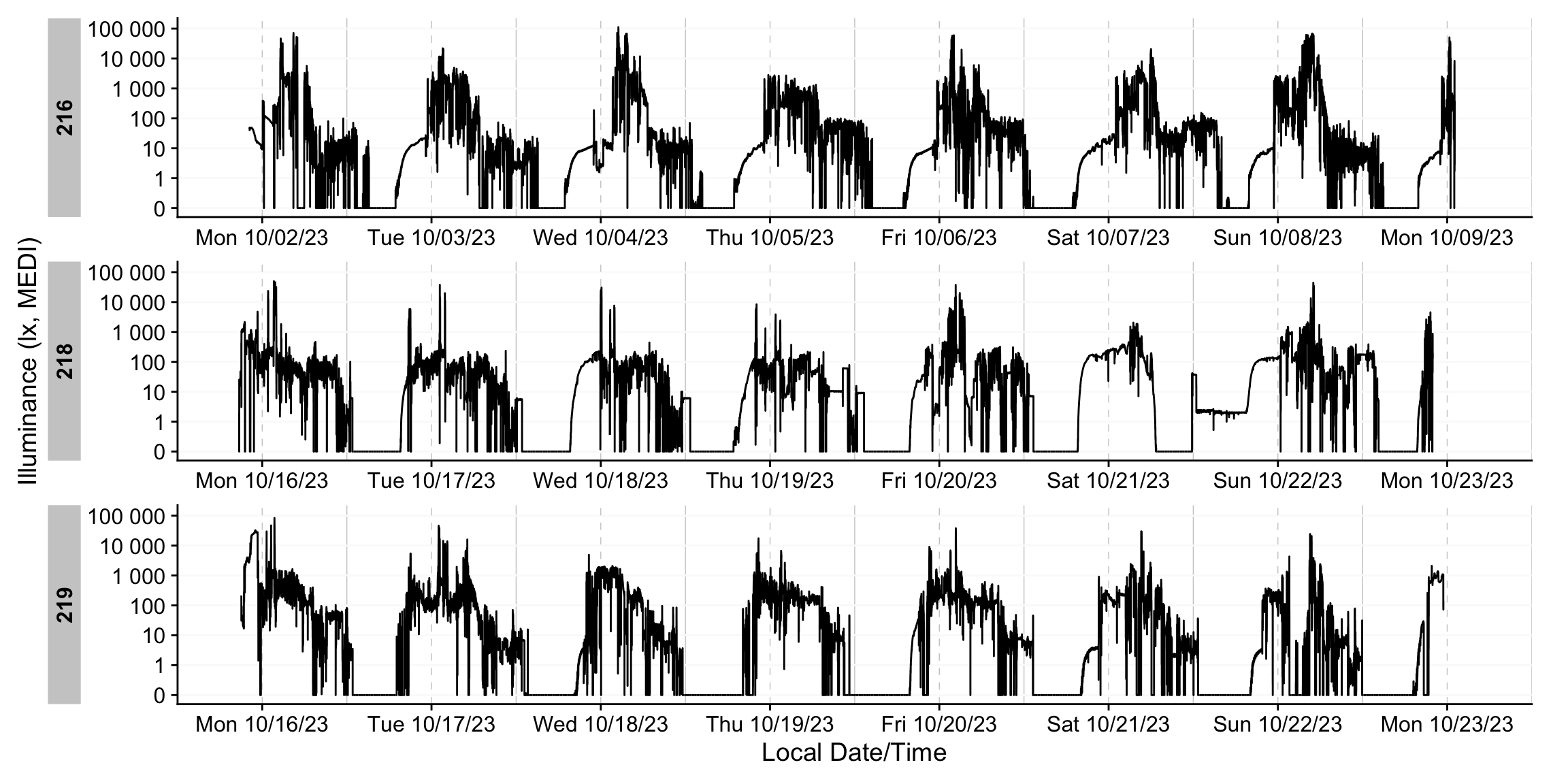
dataset_red |> gg_days()
That concludes the import section of the tutorial; next, we turn to visualization functions. For simplicitly, we will only carry a small selection of variables forward. That increases the calculation speed of many functions. Feel free to choose a different set of variables.
dataset <- dataset |> select(Id, Datetime, PIM, MEDI)How to find the correct time zone name?
A final note on imports: the function accepts only valid IANA time‑zone identifiers. You can retrieve the full list (with exact spellings) using:
OlsonNames() |> sample(5)[1] "Brazil/DeNoronha" "America/Managua" "Africa/Malabo" "Jamaica"
[5] "America/Chicago" Basic Visualizations
Visualization is central to exploratory data analysis and to communicating results in publications and presentations. LightLogR provides a suite of plotting functions built on ggplot2 and the Grammar of Graphics. As a result, the plots are composable, flexible, and straightforward to modify.
gg_days()
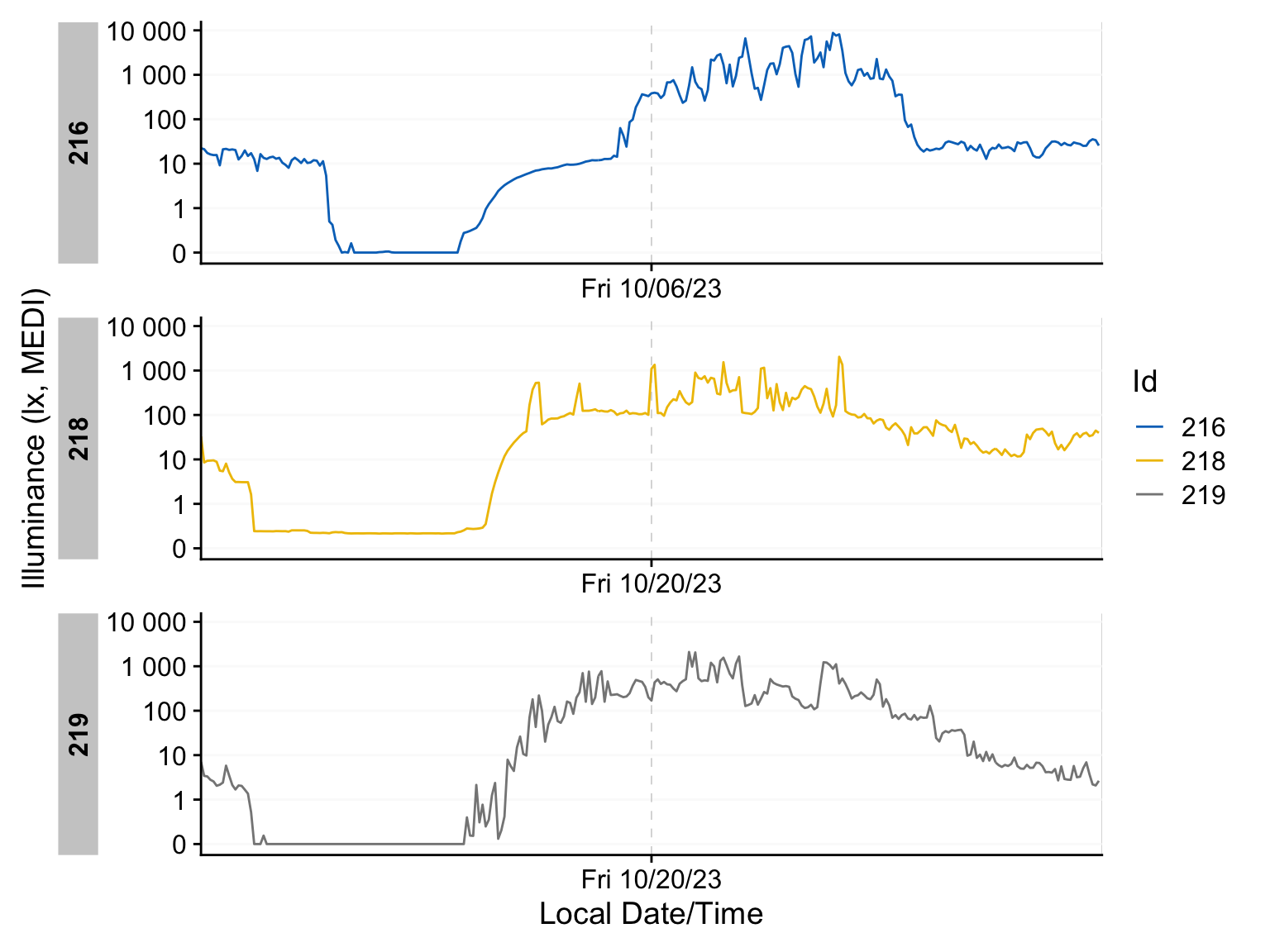
gg_days() displays a timeline per each Id. It constrains the x‑axis to complete days and, by default, uses a line geometry. The function works best for up to a handful of Id’s and 1-2 weeks of data at most.
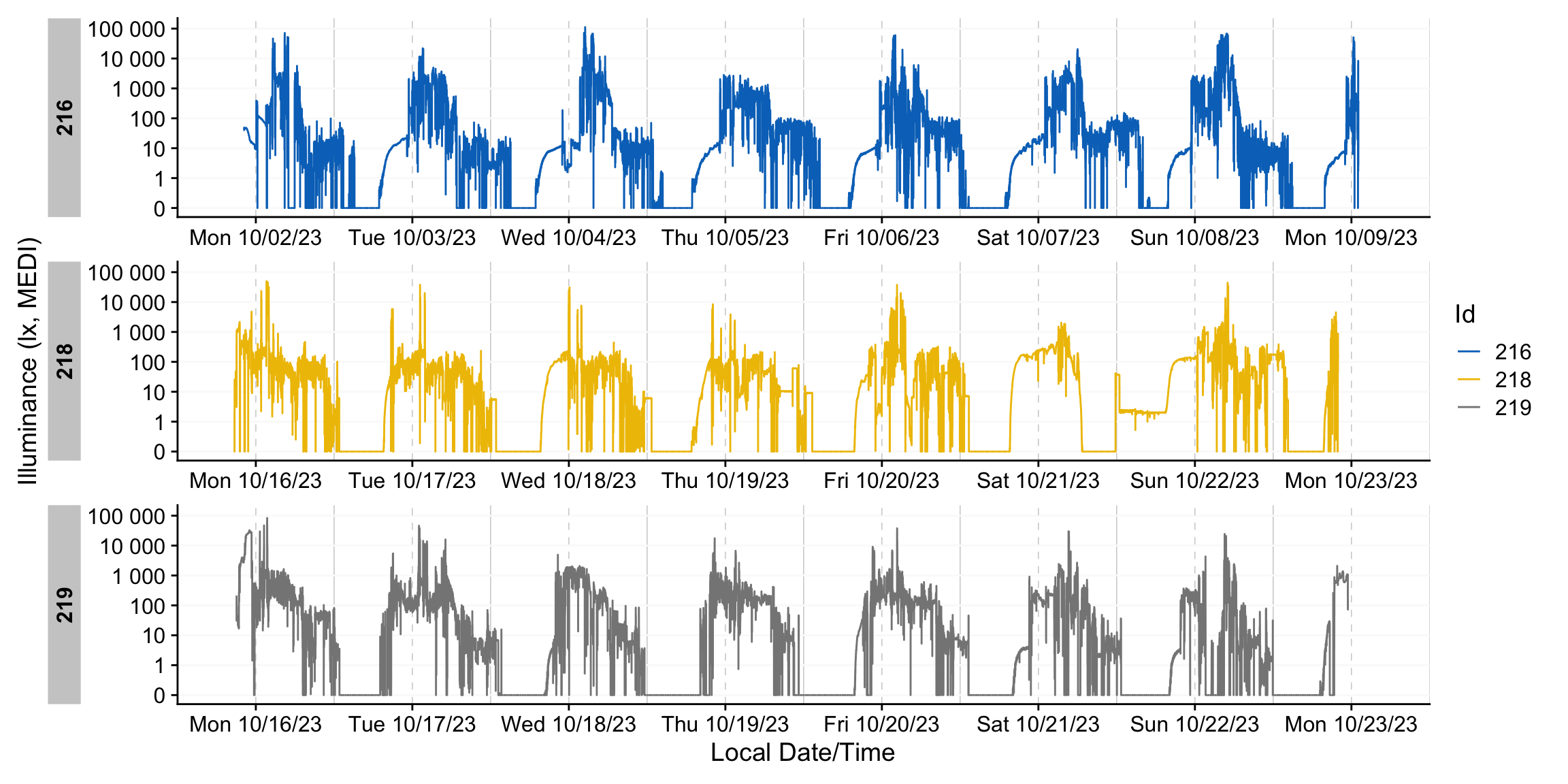
dataset_red |> gg_days(aes_col = Id) #try interactive = TRUEgg_day()
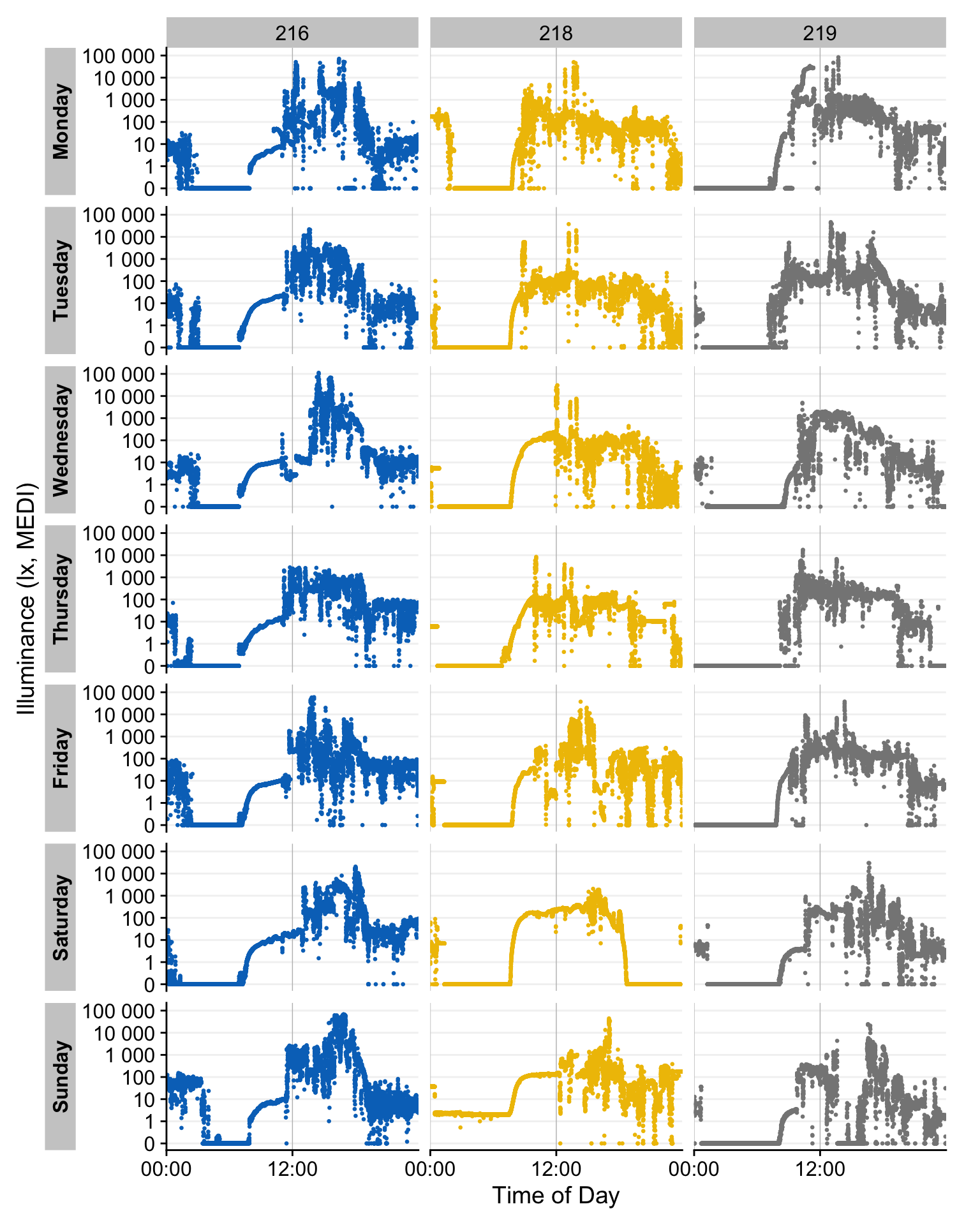
gg_day() complements gg_days() by focusing on individual calendar days. By default, it places all observations from a selected day into a single panel, regardless of source. This layout is configurable. For readability, gg_day() works best with ~1–4 days of data (at most about a week) to keep plot height manageable.
dataset_red |>
  gg_day(aes_col = Id,
         format.day = "%A", # switch from dates to week-days
         size = 0.5, # reduce point size
         x.axis.breaks = hms::hms(hours = c(0, 12))) + #12-hour grid
  guides(color = "none") + # remove color legend
  facet_grid(rows = vars(Day.data), cols = vars(Id), switch = "y") # Id x Day
gg_overview()
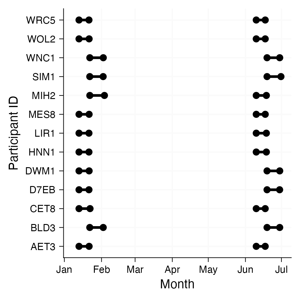
gg_overview() is invoked automatically by the import function but can also be called independently and customized. By default, each Id appears as a separate row on the y‑axis. For longitudinal datasets with large gaps between recordings, you can group observations (e.g., by a session variable) to distinguish distinct measurement periods (see margin figure). The function works nice for many participants and long collection periods, by setting their recording periods in relation. By default, it will also show times of implicitly missing data.
dataset |>
  gg_overview(col = Id) +
  ggsci::scale_color_jco() #nice color palette
gg_heatmap()
gg_heatmap() renders one calendar day per row within each data‑collection period. It is well‑suited to long monitoring spans and scales effectively to many participants. To highlight patterns that cross midnight, it supports a doubleplot option that displays a duplicate of the day, or the next day with an offset.
dataset_red |> gg_heatmap()# Looking at 5-minute bins of data
dataset_red |> gg_heatmap(unit = "5 mins")#showing data as doubleplots. Time breaks have to be reduced for legibility
dataset_red |>
gg_heatmap(doubleplot = "next",
time.breaks = c(0, 12, 24, 36, 48)*3600
)# Actogram-style heatmap (<10 lx mel EDI in this case)
dataset_red |>
gg_heatmap(MEDI < 10,
doubleplot = "next",
time.breaks = c(0, 12, 24, 36, 48)*3600,
fill.limits = c(0, NA),
fill.remove = TRUE,
fill.title = "<10lx mel EDI"
) +
scale_fill_manual(values = c("TRUE" = "black", "FALSE" = "#00000000"))What about non-light variables?
LightLogR is optimized for wearable light sensors and selects sensible defaults: for example, melanopic EDI (when available) and settings suited to typical light‑exposure distributions. Nevertheless, the functions are measurement‑agnostic and can be applied to non‑light variables. Consult the function documentation to see which arguments to adjust for your variable of interest. For example, here we plot an activity variable:
dataset_red |>
  gg_days(
    y.axis = PIM, #variable PIM
    y.scale = "identity", #set a linear scale
    y.axis.breaks = waiver(), #choose standard axis breaks according to values
    y.axis.label = "Proportional integration mode (PIM)"
  ) +
  coord_cartesian(ylim = c(0, 5000))
Validation
Currently, LightLogR’s validation aims to ensure a regular, uninterrupted time series for each participant. Additional features are planned.
The figures at the side summarize the gap terminology used in LightLogR and illustrate how gap_handler() fills implicit missing data.
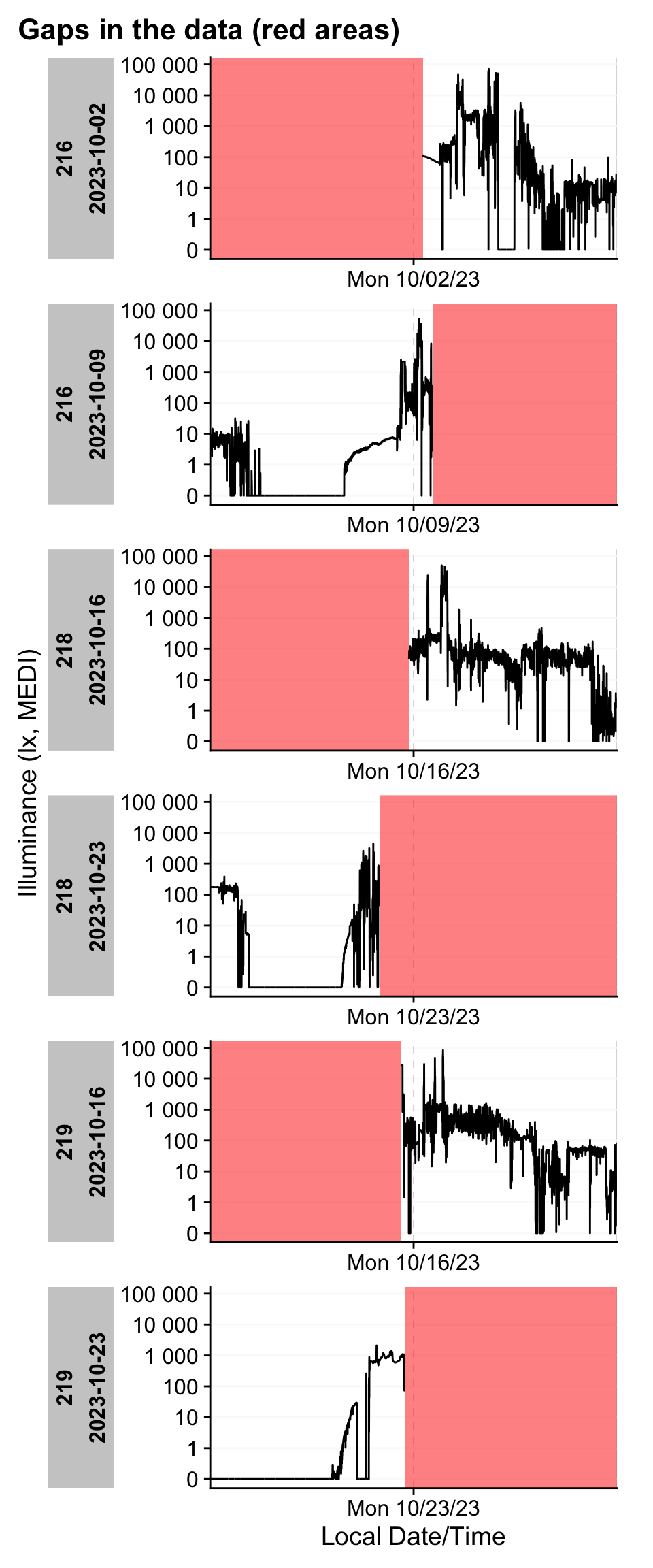
gap_handler() identifies the time series’ dominant epoch (the most common sampling interval) and fills NA entries between the first and last observation. By default, no observations are dropped, so irregular samples are preserved.To quickly assess whether a dataset contains (implicit) gaps or irregular sampling, use the following diagnostic helpers:
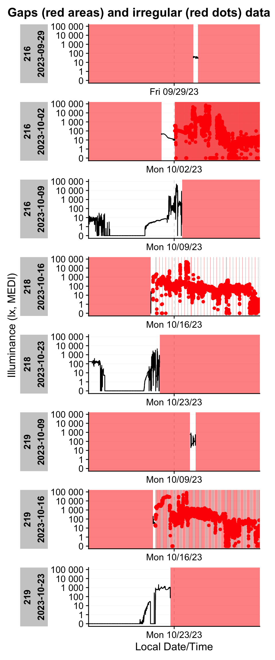
We can then quickly visualize where these issues occur within the affected days.
dataset |> gg_gaps(group.by.days = TRUE, show.irregulars = TRUE)This function can be slow when a dataset contains many gaps or irregular samples. If needed, pre‑filter the data or adjust the function’s arguments.
In our example, we identify eight participant‑days with gaps:
- Three straightforward cases: data collection ends around noon on Monday, leaving the remainder of the day missing. By default, the function evaluates complete calendar days (this is configurable). These days only require converting implicit gaps into explicit missing values.
- Two pre‑trial snippets: brief measurements occur on the Friday or Monday preceding the trial—likely test recordings. These days are outside the study window and should be removed entirely.
- Three early irregularities: irregular sampling appears shortly after data collection starts. This most likely reflects a test recording immediately before the device was handed to the participant. Trimming this initial segment eliminates the irregularity and the rest of the day can be changed to explicit missingness.
Preparing the dataset
There are several ways to address these issues. We will showcase three in the next sections.
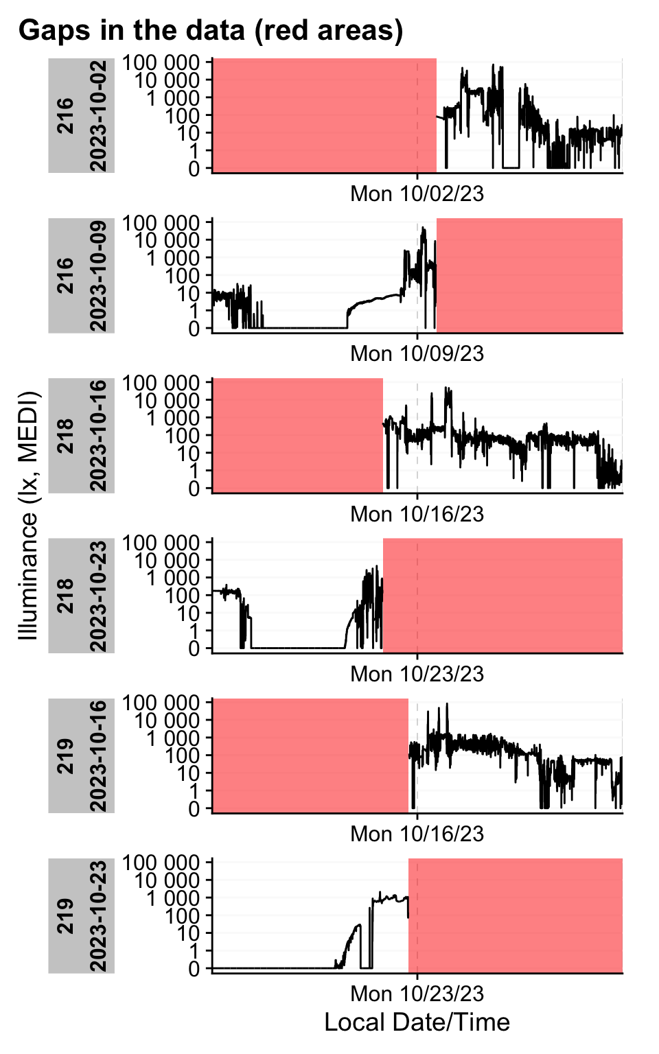
1. Set the maximum length of the dataset.
If the study follows a fixed‑length protocol, you can enforce a maximum observation window (e.g., 7 days) by trimming from the beginning so that each participant’s series has the same duration. This approach preserves participant‑specific end times, which must meaningfully reflect protocol completion; otherwise, you risk cutting away valid data.
dataset |>
filter_Datetime(length = "7 days", length_from_start = FALSE) |>
  gg_gaps(group.by.days = TRUE, show.irregulars = TRUE)
The remaining gaps are simple start‑ and end‑day truncations.
2. Remove the first values from the dataset
You can remove a fixed number of observations from the beginning of each participant’s series. This approach is helpful when the exact total measurement duration is not critical—for example, to discard brief pre‑trial test recordings or initial device‑stabilization periods.
dataset |>
  slice_tail(n = -(3*60*6)) |>
  gg_gaps(group.by.days = TRUE, show.irregulars = TRUE)
The results are similarly effective.
3. Trim with a list
The most robust way to enforce sensible measurement windows is to supply a table of trial start and end timestamps (per participant) and filter the time series accordingly. In this tutorial we create that table on the fly; in practice, it is typically stored in a CSV or Excel file. The add_states() function provides an effective interface between the two datasets: it aligns by identifier and time, adds state information (e.g., “in‑trial”), and enables precise trimming. Ensure that the identifying variables (e.g., Id) are named identically across files.
#create a dataframe of trial times
trial_times <-
  data.frame(
    Id = c("216", "218", "219"),
    start = c(
      "02.10.2023  12:30:00",
      "16.10.2023  12:00:00",
      "16.10.2023  12:00:00"
    ),
    end = c(
      "09.10.2023  12:30:00",
      "23.10.2023  12:00:00",
      "23.10.2023  12:00:00"
    ),
    trial = TRUE
  ) |>
  mutate(across(
    c(start, end),
    \(x) parse_date_time(x, order = "%d%m%y %H%M%S", tz = "Europe/Berlin")
  )) |>
  group_by(Id)
# filter dataset by trial time
dataset <-
dataset |>
add_states(trial_times) |>
dplyr::filter(trial) |>
select(-trial)
dataset |>
gg_gaps(group.by.days = TRUE, show.irregulars = TRUE)gap_table()
We can summarize each dataset’s regularity and missingness in a table. Note that this function may be slow when many gaps are present.
| Summary of available and missing data | |||||||||||||
| Variable: melanopic EDI | |||||||||||||
Data
|
Missing
|
||||||||||||
|---|---|---|---|---|---|---|---|---|---|---|---|---|---|
Regular
|
Irregular
|
Range
|
Interval
|
Gaps
|
Implicit
|
Explicit
|
|||||||
| Time | % | n1,2 | Time | Time | N | ø | Time | % | Time | % | Time | % | |
| Overall | 2w 6d 21h 28m 10s | 87.1%3 | 0 | 3w 3d | 10 | 6 | 1d 13h 15m 55s | 3d 2h 31m 50s | 12.9%3 | 3d 2h 31m 50s | 12.9%3 | 0s | 0.0%3 |
| 216 | |||||||||||||
| 1w | 87.5% | 0 | 1w 1d | 10s | 2 | 12h | 1d | 12.5% | 1d | 12.5% | 0s | 0.0% | |
| 218 | |||||||||||||
| 6d 21h 58m 50s | 86.4% | 0 | 1w 1d | 10s | 2 | 13h 35s | 1d 2h 1m 10s | 13.6% | 1d 2h 1m 10s | 13.6% | 0s | 0.0% | |
| 219 | |||||||||||||
| 6d 23h 29m 20s | 87.2% | 0 | 1w 1d | 10s | 2 | 12h 15m 20s | 1d 30m 40s | 12.8% | 1d 30m 40s | 12.8% | 0s | 0.0% | |
| 1 If n > 0: it is possible that the other summary statistics are affected, as they are calculated based on the most prominent interval. | |||||||||||||
| 2 Number of (missing or actual) observations | |||||||||||||
| 3 Based on times, not necessarily number of observations | |||||||||||||
gap_handler()
Approximately 13% of the missing data are implicit—they arise from truncated start and end days. It is good practice to make these gaps explicit. Use gap_handler(full.days = TRUE) to fill implicit gaps to full‑day regularity. Then verify the result with gap_table(), the diagnostic helpers, and a follow‑up visualization:
dataset <- dataset |> gap_handler(full.days = TRUE)
dataset |> gap_table() |> cols_hide(contains("_n"))| Summary of available and missing data | |||||||||||||
| Variable: melanopic EDI | |||||||||||||
Data
|
Missing
|
||||||||||||
|---|---|---|---|---|---|---|---|---|---|---|---|---|---|
Regular
|
Irregular
|
Range
|
Interval
|
Gaps
|
Implicit
|
Explicit
|
|||||||
| Time | % | n1,2 | Time | Time | N | ø | Time | % | Time | % | Time | % | |
| Overall | 2w 6d 21h 28m 10s | 87.1%3 | 0 | 3w 3d | 10 | 6 | 1d 13h 15m 55s | 3d 2h 31m 50s | 12.9%3 | 0s | 0.0%3 | 3d 2h 31m 50s | 12.9%3 |
| 216 | |||||||||||||
| 1w | 87.5% | 0 | 1w 1d | 10s | 2 | 12h | 1d | 12.5% | 0s | 0.0% | 1d | 12.5% | |
| 218 | |||||||||||||
| 6d 21h 58m 50s | 86.4% | 0 | 1w 1d | 10s | 2 | 13h 35s | 1d 2h 1m 10s | 13.6% | 0s | 0.0% | 1d 2h 1m 10s | 13.6% | |
| 219 | |||||||||||||
| 6d 23h 29m 20s | 87.2% | 0 | 1w 1d | 10s | 2 | 12h 15m 20s | 1d 30m 40s | 12.8% | 0s | 0.0% | 1d 30m 40s | 12.8% | |
| 1 If n > 0: it is possible that the other summary statistics are affected, as they are calculated based on the most prominent interval. | |||||||||||||
| 2 Number of (missing or actual) observations | |||||||||||||
| 3 Based on times, not necessarily number of observations | |||||||||||||
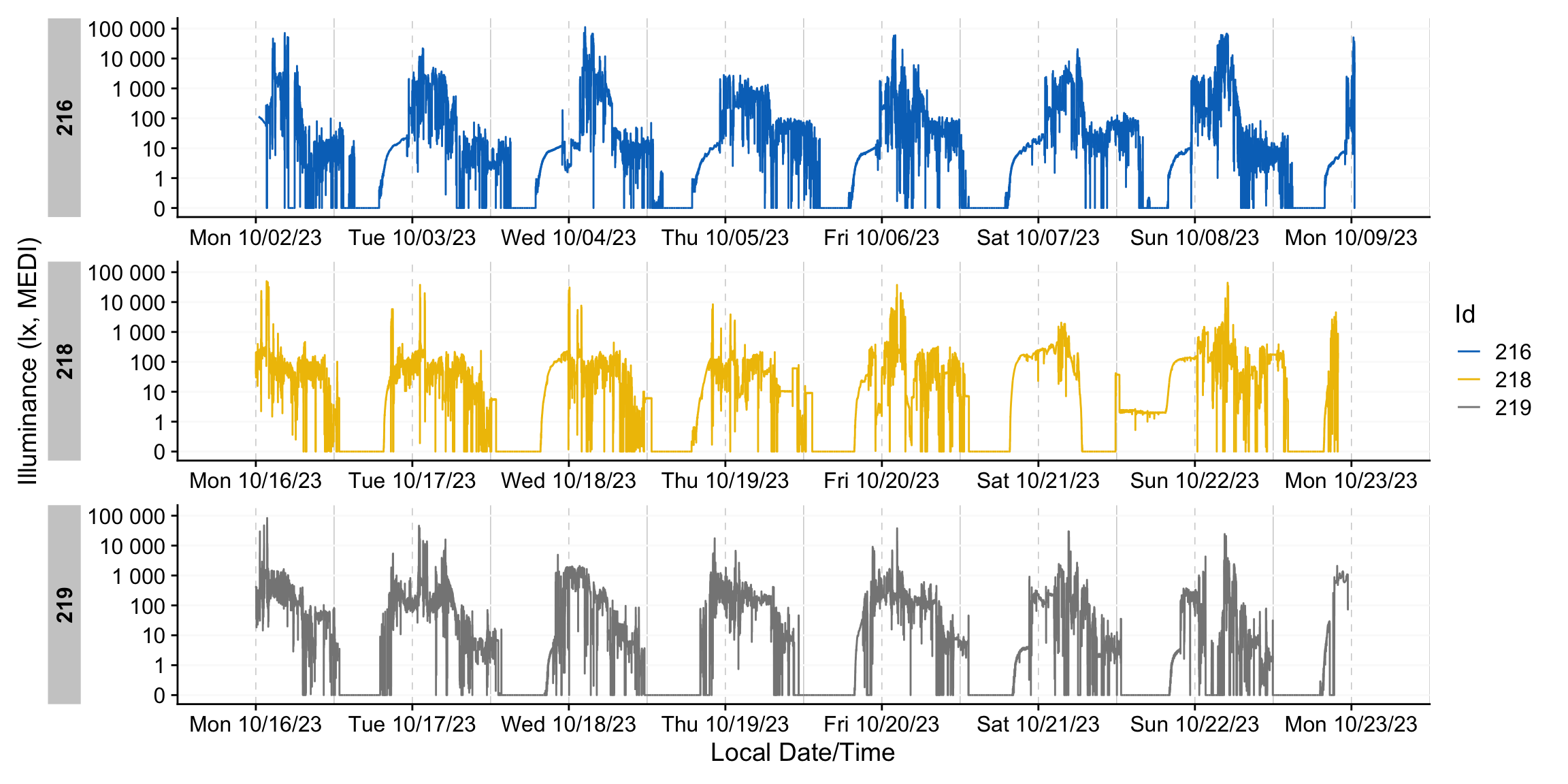
dataset |> gg_days(aes_col = Id)remove_partial_data()
It is often necessary to set missingness thresholds at different levels (hour, day, participant). Typical questions include:
- How much data may be missing within an hour before that hour is excluded?
- How much data may be missing from a day before that day is excluded?
- How much data may be missing for a participant before excluding them from further analyses?
remove_partial_data() addresses these questions. It evaluates each group (by default, Id) and quantifies missingness either as an absolute duration or a relative proportion. Groups that exceed the specified threshold are discarded. A useful option is by.date, which performs the thresholding per calendar day (for removal) while leaving the output grouping unchanged. Note that missingness is determined by the amount of data points in each group, relative to NA values.
For this tutorial, we will remove any day with more than one hour of missing data—this effectively drops both partial Mondays:
dataset <-
  dataset |>
  remove_partial_data(Variable.colname = MEDI,
                      threshold.missing = "1 hour",
                      by.date = TRUE)

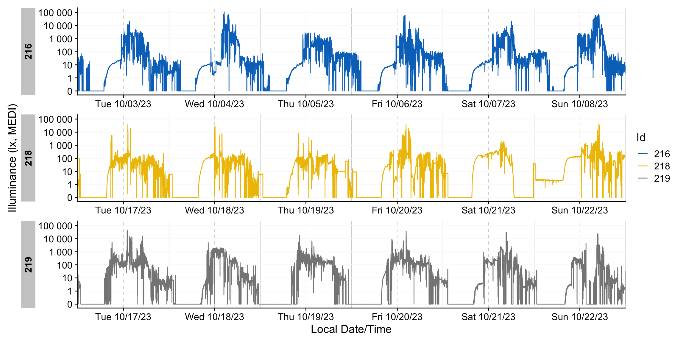
dataset |> gg_days(aes_col = Id)Why did we just spend all this time handling gaps and irregularities on the Mondays only to remove them afterward?
Not all datasets are this straightforward. Deciding whether a day should be included in the analysis should come after ensuring the data are aligned to a regular, uninterrupted time series. Regularization makes diagnostics meaningful and prevents threshold rules from behaving unpredictably.
Moreover, there are different frameworks for grouping personal light‑exposure data. In this tutorial we focus on calendar dates and 24‑hour days. Other frameworks group differently. For example, anchoring to sleep–wake cycles—under which both Mondays might still contain useful nocturnal data. Harmonizing first ensures those alternatives remain viable even if calendar‑day summaries are later excluded.
Metrics
Metrics form the second major pillar of LightLogR, alongside visualization. The literature contains many light‑exposure metrics; LightLogR implements a broad set of them behind a uniform, well‑documented interface. The currently available metrics are:
| Metric Family | Submetrics | Note | Documentation |
|---|---|---|---|
| Barroso | 7 | barroso_lighting_metrics() |
|
| Bright-dark period | 4x2 | bright / dark | bright_dark_period() |
| Centroid of light exposure | 1 | centroidLE() |
|
| Dose | 1 | dose() |
|
| Disparity index | 1 | disparity_index() |
|
| Duration above threshold | 3 | above, below, within | duration_above_threshold() |
| Exponential moving average (EMA) | 1 | exponential_moving_average() |
|
| Frequency crossing threshold | 1 | frequency_crossing_threshold() |
|
| Intradaily Variance (IV) | 1 | intradaily_variability() |
|
| Interdaily Stability (IS) | 1 | interdaily_stability() |
|
| Midpoint CE (Cumulative Exposure) | 1 | midpointCE() |
|
| nvRC (Non-visual circadian response) | 4 |
nvRC(), nvRC_circadianDisturbance(), nvRC_circadianBias(), nvRC_relativeAmplitudeError()
|
|
| nvRD (Non-visual direct response) | 2 |
nvRD(), nvRD_cumulative_response()
|
|
| Period above threshold | 3 | above, below, within | period_above_threshold() |
| Pulses above threshold | 7x3 | above, below, within | pulses_above_threshold() |
| Threshold for duration | 2 | above, below | threshold_for_duration() |
| Timing above threshold | 3 | above, below, within | timing_above_threshold() |
| Total: | |||
| 17 families | 62 metrics |
LightLogR supports a wide range of metrics across different metric families. You can find the full documentation of metrics functions in the reference section. There is also an overview article on how to use Metrics.
If you would like to use a metric you don’t find represented in LightLogR, please contact the developers. The easiest and most trackable way to get in contact is by opening a new issue on our Github repository.
Principles
Each metric function operates on vectors. Although the main argument is often named Light.vector, the name is conventional - the function will accept any variable you supply. All metric functions are thoroughly documented, with references to their intended use and interpretation.
While we don’t generally recommend it, you can pass a raw vector directly to a metric function. For example, to compute Time above 250 lx melanopic EDI, you could run:
duration_above_threshold(
  Light.vector = dataset$MEDI,
  Time.vector = dataset$Datetime,
  threshold = 250
)
[1] "179840s (~2.08 days)"However, that single result is not very informative - it aggregates across all participants and all days. To recover the total recorded duration, recompute the complementary metric: Time below 250 lx melanopic EDI. This should approximate the full two weeks and four days of data when evaluated over the whole dataset:
duration_above_threshold(
  Light.vector = dataset$MEDI,
  Time.vector = dataset$Datetime,
  threshold = 250,
  comparison = "below"
)
[1] "1375360s (~2.27 weeks)"The problem is amplified for metrics defined at the day scale (or shorter). For example, the brightest 10 hours (M10) is computed within each 24‑hour day using a consecutive 10‑hour window—so applying it to a pooled, cross‑day vector is almost meaningless:
bright_dark_period(
  Light.vector = dataset$MEDI,
  Time.vector = dataset$Datetime,
  as.df = TRUE
) |>
  gt() |> tab_header("M10")
Warning in bright_dark_period(Light.vector = dataset$MEDI, Time.vector =
dataset$Datetime, : `Time.vector` is not regularly spaced. Calculated results
may be incorrect!| M10 | |||
| brightest_10h_mean | brightest_10h_midpoint | brightest_10h_onset | brightest_10h_offset |
|---|---|---|---|
| 3292.002 | 2023-10-08 15:17:49 | 2023-10-08 10:17:59 | 2023-10-08 20:17:49 |
The resulting value - although computationally valid - is substantively meaningless: it selects the single brightest 10‑hour window across all participants, rather than computing M10 per participant per day. In addition, two time series (218 & 219) overlap in time, which violates the assumption of a single, regularly spaced series and can produce errors. Hence the Warning: Time.vector is not regularly spaced. Calculated results may be incorrect!
Accordingly, metric functions should be applied within tidy groups (e.g., by Id and by calendar Date), not to a pooled vector. You can achieve this with explicit for‑loops or, preferably, a tidy approach using dplyr (e.g., group_by()/summarise() or nest()/map()). We recommend the latter.
Use of summarize()
Wrap the metric inside a dplyr summarise()/summarize() call, supply the grouped dataset, and set as.df = TRUE. This yields a tidy, one‑row‑per‑group result (e.g., per Id). For example, computing interdaily stability (IS):
dataset |>
  summarize(
    interdaily_stability(
      Light.vector = MEDI,
      Datetime.vector = Datetime,
      as.df = TRUE
    )
  )
# A tibble: 3 × 2
Id interdaily_stability
<chr> <dbl>
1 216 0.260
2 218 0.339
3 219 0.389To compute multiple metrics at once, include additional expressions inside the summarize() call. For instance, add Time above 250 lx melanopic EDI alongside IS:
dataset |>
  summarize(
     duration_above_threshold(
      Light.vector = MEDI,
      Time.vector = Datetime,
      threshold = 250,
      as.df = TRUE
    ),
    interdaily_stability(
      Light.vector = MEDI,
      Datetime.vector = Datetime,
      as.df = TRUE
    )
  )
# A tibble: 3 × 3
Id duration_above_250 interdaily_stability
<chr> <Duration> <dbl>
1 216 89160s (~1.03 days) 0.260
2 218 31160s (~8.66 hours) 0.339
3 219 59520s (~16.53 hours) 0.389For finer granularity, add additional grouping variables before summarizing—for example, group by calendar Date to compute metrics per participant–day:
TAT250 <-
dataset |>
  add_Date_col(group.by = TRUE, as.wday = TRUE) |> #add a Date column + group
    summarize(
     duration_above_threshold(
      Light.vector = MEDI,
      Time.vector = Datetime,
      threshold = 250,
      as.df = TRUE
    ),
    .groups = "drop_last"
  )

TAT250 |> gt()| Date | duration_above_250 |
|---|---|
| 216 | |
| Tue | 15360s (~4.27 hours) |
| Wed | 14910s (~4.14 hours) |
| Thu | 17550s (~4.88 hours) |
| Fri | 9900s (~2.75 hours) |
| Sat | 12180s (~3.38 hours) |
| Sun | 19260s (~5.35 hours) |
| 218 | |
| Tue | 1900s (~31.67 minutes) |
| Wed | 1080s (~18 minutes) |
| Thu | 760s (~12.67 minutes) |
| Fri | 6170s (~1.71 hours) |
| Sat | 10370s (~2.88 hours) |
| Sun | 10880s (~3.02 hours) |
| 219 | |
| Tue | 12250s (~3.4 hours) |
| Wed | 14400s (~4 hours) |
| Thu | 10200s (~2.83 hours) |
| Fri | 8940s (~2.48 hours) |
| Sat | 5820s (~1.62 hours) |
| Sun | 7910s (~2.2 hours) |
We can further condense this:
TAT250 |>
  summarize_numeric() |>
gt()| Id | mean_duration_above_250 | episodes |
|---|---|---|
| 216 | 14860s (~4.13 hours) | 6 |
| 218 | 5193s (~1.44 hours) | 6 |
| 219 | 9920s (~2.76 hours) | 6 |
That’s all you need to get started with metric calculation in LightLogR. While advanced metrics involve additional considerations, this tidy grouped workflow will take you a long way.
Photoperiod
Photoperiod is a key covariate in many analyses of personal light exposure. LightLogR includes utilities to derive photoperiod information with minimal effort. All you need are geographic coordinates in decimal degrees (latitude, longitude); functions will align photoperiod features to your time series. Provide coordinates in standard decimal format (e.g., 48.52, 9.06):
#specifying coordinates (latitude/longitude)
coordinates <- c(48.521637, 9.057645)

#extracting photoperiod information
dataset |> extract_photoperiod(coordinates)
date tz lat lon solar.angle dawn
1 2023-10-03 Europe/Berlin 48.52164 9.057645 -6 2023-10-03 06:54:12
2 2023-10-04 Europe/Berlin 48.52164 9.057645 -6 2023-10-04 06:55:38
3 2023-10-05 Europe/Berlin 48.52164 9.057645 -6 2023-10-05 06:57:04
4 2023-10-06 Europe/Berlin 48.52164 9.057645 -6 2023-10-06 06:58:30
5 2023-10-07 Europe/Berlin 48.52164 9.057645 -6 2023-10-07 06:59:56
6 2023-10-08 Europe/Berlin 48.52164 9.057645 -6 2023-10-08 07:01:22
7 2023-10-17 Europe/Berlin 48.52164 9.057645 -6 2023-10-17 07:14:23
8 2023-10-18 Europe/Berlin 48.52164 9.057645 -6 2023-10-18 07:15:50
9 2023-10-19 Europe/Berlin 48.52164 9.057645 -6 2023-10-19 07:17:17
10 2023-10-20 Europe/Berlin 48.52164 9.057645 -6 2023-10-20 07:18:45
11 2023-10-21 Europe/Berlin 48.52164 9.057645 -6 2023-10-21 07:20:13
12 2023-10-22 Europe/Berlin 48.52164 9.057645 -6 2023-10-22 07:21:40
dusk photoperiod
1 2023-10-03 19:30:44 12.60884 hours
2 2023-10-04 19:28:41 12.55080 hours
3 2023-10-05 19:26:39 12.49293 hours
4 2023-10-06 19:24:37 12.43521 hours
5 2023-10-07 19:22:36 12.37767 hours
6 2023-10-08 19:20:35 12.32031 hours
7 2023-10-17 19:03:11 11.81335 hours
8 2023-10-18 19:01:19 11.75821 hours
9 2023-10-19 18:59:29 11.70333 hours
10 2023-10-20 18:57:40 11.64874 hours
11 2023-10-21 18:55:53 11.59443 hours
12 2023-10-22 18:54:06 11.54043 hours#adding photoperiod information
dataset <-
dataset |>
add_photoperiod(coordinates)
dataset |> head()# A tibble: 6 × 9
# Groups: Id [1]
Id Datetime is.implicit PIM MEDI dawn
<chr> <dttm> <lgl> <dbl> <dbl> <dttm>
1 216 2023-10-03 00:00:09 FALSE 91 12.6 2023-10-03 06:54:12
2 216 2023-10-03 00:00:19 FALSE 62 14.3 2023-10-03 06:54:12
3 216 2023-10-03 00:00:29 FALSE 45 10.2 2023-10-03 06:54:12
4 216 2023-10-03 00:00:39 FALSE 13 10.3 2023-10-03 06:54:12
5 216 2023-10-03 00:00:49 FALSE 216 11.9 2023-10-03 06:54:12
6 216 2023-10-03 00:00:59 FALSE 62 11.6 2023-10-03 06:54:12
# ℹ 3 more variables: dusk <dttm>, photoperiod <drtn>, photoperiod.state <chr>Photoperiod in visualizations
#if photoperiod information was already added to the data
#nothing has to be specified
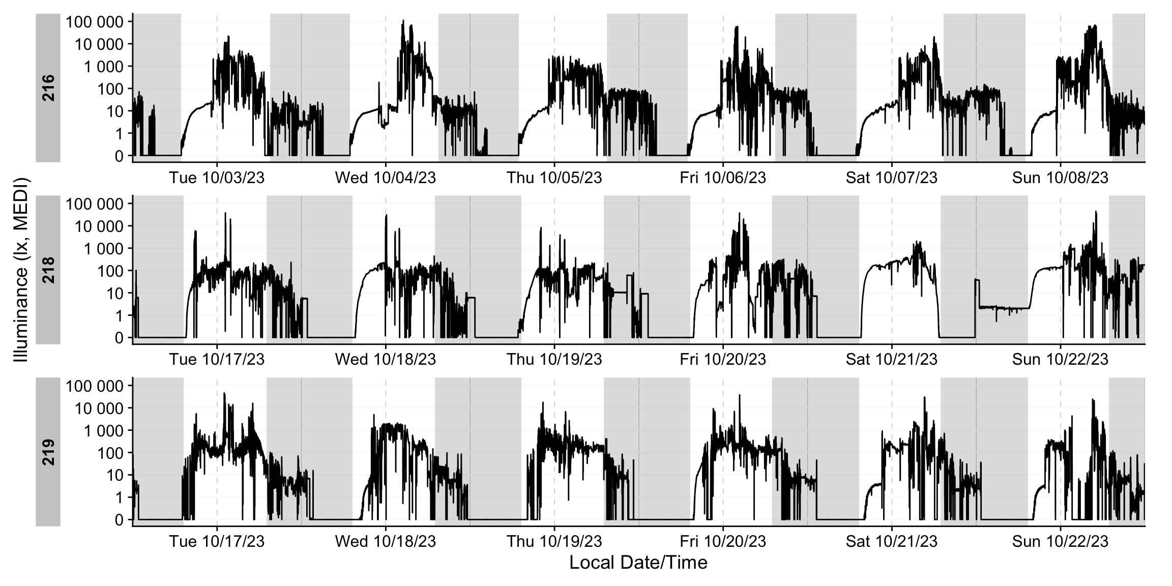
dataset |> gg_days() |> gg_photoperiod()
#if no photoperiod information is available in the data, coordinates have to
#be specified
dataset_red |> gg_days() |> gg_photoperiod(coordinates)Data
Photoperiod features make it easy to split data into day and night states—for example, to compute metrics by phase. The number_states() function places a counter each time the state changes, effectively numbering successive day and night episodes. Grouping by these counters then allows you to calculate metrics for individual days and nights:
dataset |>
  #create numbered days and nights:
  number_states(photoperiod.state) |>
  #group by Id, day and nights, and also the numbers:
  group_by(photoperiod.state, photoperiod.state.count, .add = TRUE) |>
  #calculate the brightest hour in each day and each night:
  summarize(
    bright_dark_period(MEDI, Datetime, timespan = "1 hour", as.df = TRUE),
    .groups = "drop_last") |>
  #select (bright_dark_period calulates four metrics: start, end, middle, mean)
  select(Id, photoperiod.state, brightest_1h_mean) |>
  #condense the instances to a single summary
  summarize_numeric(prefix = "") |>
  #show as table
gt() |> fmt_number()| photoperiod.state | brightest_1h_mean | episodes |
|---|---|---|
| 216 | ||
| day | 7,294.36 | 6.00 |
| night | 34.87 | 7.00 |
| 218 | ||
| day | 1,246.30 | 6.00 |
| night | 72.96 | 7.00 |
| 219 | ||
| day | 1,670.66 | 6.00 |
| night | 51.40 | 7.00 |
This yields the average brightest 1‑hour period for each participant, separately for day and night. Notably, the participant with the highest daytime brightness also shows the lowest nighttime brightness, and vice versa.
Distribution of light exposure
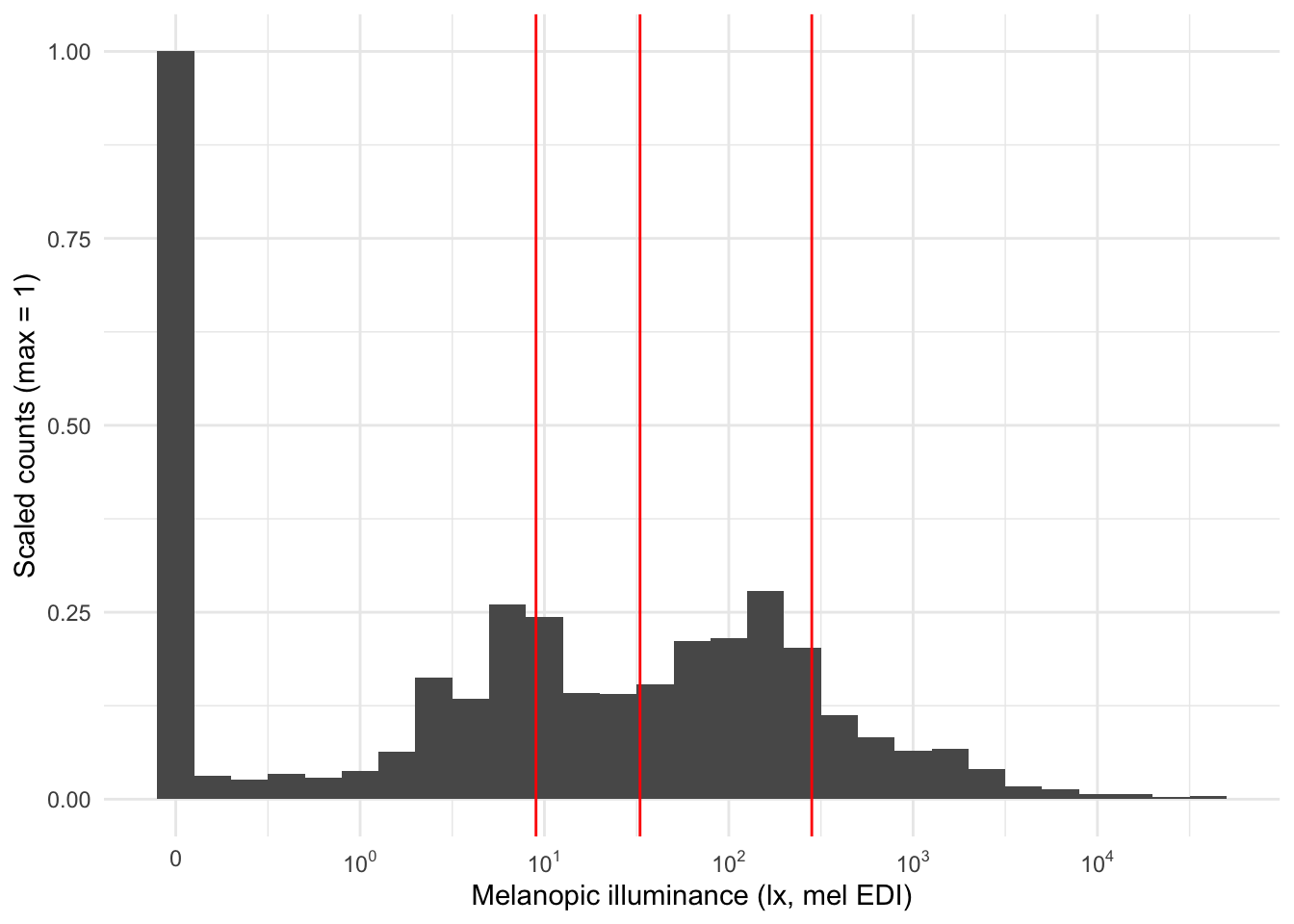
Personal light‑exposure data exhibit a characteristic distribution (see figure): they are strongly right‑skewed—approximately log‑normal—and contain many zeros (i.e., zero‑inflation).
Consequently, the arithmetic mean is not a representative summary for these data. We can visualize this by placing common location metrics on the distribution.
| mean | median | geo_mean |
|---|---|---|
| 282.535 | 8.76 | 32.82594 |
dataset |>
  aggregate_Datetime("5 min") |>
  ggplot(aes(x=MEDI, y = after_stat(ncount))) +
  geom_histogram(binwidth = 0.2) +
  scale_x_continuous(trans = "symlog",
                     breaks = c(0, 10^(0:5)),
                     labels= expression(0,10^0,10^1, 10^2, 10^3, 10^4, 10^5)
                     ) +
  geom_vline(xintercept = c(282, 9, 33), col = "red") +
  theme_minimal() +
  # facet_wrap(~Id) +
  labs(x = "Melanopic illuminance (lx, mel EDI)", y = "Scaled counts (max = 1)")
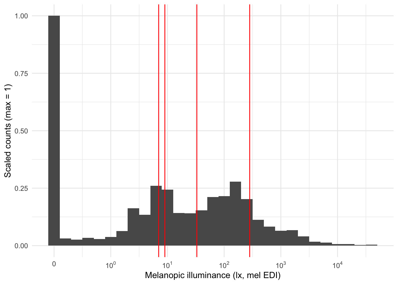
To better characterize zero‑inflated, right‑skewed light data, use log_zero_inflated(). The function adds a small constant (ε) to every observation before taking logs, making the transform well‑defined at zero. Choose ε based on the device’s measurement resolution/accuracy; for wearables spanning roughly 1–10^5 lx, we recommend ε = 0.1 lx. The inverse, exp_zero_inflated(), returns values to the original scale by exponentiating and then subtracting the same ε. The default basis for these functions is 10.
| mean | median | geo_mean | log_zero_inflated_mean |
|---|---|---|---|
| 282.535 | 8.76 | 32.82594 | 6.567388 |
dataset |>
  aggregate_Datetime("5 min") |>
  ggplot(aes(x=MEDI, y = after_stat(ncount))) +
  geom_histogram(binwidth = 0.2) +
  scale_x_continuous(trans = "symlog",
                     breaks = c(0, 10^(0:5)),
                     labels= expression(0,10^0,10^1, 10^2, 10^3, 10^4, 10^5)
                     ) +
  geom_vline(xintercept = c(282, 9, 33, 7), col = "red") +
  theme_minimal() +
  # facet_wrap(~Id) +
  labs(x = "Melanopic illuminance (lx, mel EDI)", y = "Scaled counts (max = 1)")
Log zero-inflated with metrics
When computing averaging metrics, apply the transformation explicitly to the variable you pass to the metric. This ensures the statistic is computed on the intended scale and makes your code easy to audit later.
For the zero‑inflated log approach, transform before averaging and (if desired) back‑transform for reporting:
dataset |>
  filter(Id == "216") |>
  add_Date_col(group.by = TRUE) |>
  summarize(
    #without transformation:
    bright_dark_period(MEDI, Datetime, as.df = TRUE),
    #with transformation:
    bright_dark_period(
      log_zero_inflated(MEDI),
      timespan = "9.99 hours", #needs to be different from 10 or it overwrites
      Datetime, as.df = TRUE),
    .groups = "drop_last"
            ) |>
  select(Id, Date, brightest_10h_mean, brightest_9.99h_mean) |>
  mutate(brightest_9.99h_mean = exp_zero_inflated(brightest_9.99h_mean)) |>
  rename(brightest_10h_zero_infl_mean = brightest_9.99h_mean) |>
  gt() |>
fmt_number()| Date | brightest_10h_mean | brightest_10h_zero_infl_mean |
|---|---|---|
| 216 | ||
| 2023-10-03 | 774.39 | 164.46 |
| 2023-10-04 | 1,890.69 | 106.63 |
| 2023-10-05 | 355.81 | 153.26 |
| 2023-10-06 | 706.41 | 117.82 |
| 2023-10-07 | 790.83 | 125.38 |
| 2023-10-08 | 3,292.00 | 250.35 |
Summaries
Summary helpers provide fast, dataset‑wide overviews. Existing examples include gap_table() (tabular diagnostics) and gg_overview() (visual timeline). In the next release, a higher‑level tool is planned: grand_overview() (a dataset‑level summary plot). Already implemented in LightLogR 0.10.0 is summary_table() (a table of key exposure metrics). In keeping with LightLogR’s design, they have straightforward interfaces and play well with grouped/tidy workflows.
Summary plot
dataset |>
  grand_overview(coordinates, #provide the coordinates
                 "Tübingen", #provide a site name
                 "Germany", #provide a country name
                 "#DDCC77", #provide a color for the dataset
                 photoperiod_sequence = 1 #specify the photoperiod resolution
                 )
# ggsave("assets/grand_overview.png", width = 17, height = 10, scale = 2, units = "cm")Summary table
summary_table <-
dataset |>
summary_table(
  coordinates = coordinates, #provide coordinates
  location = "Tuebingen", #provide a site name
  site = "Germany", #provide a country name
  color = "#DDCC77", #provide a color for histograms
  histograms = TRUE #show histograms
)

summary_table | Summary table | ||||
| Tuebingen, Germany, 48.5°N, 9.1°E, TZ: Europe/Berlin | ||||
| Overview | ||||
|---|---|---|---|---|
| Participants | Participants | 3 | ||
| Participant-days | Participant-days | 18 (6 - 6) | ||
| Days ≥80% complete | Days ≥80% complete | 18 (6 - 6) | ||
| Missing/irregular | Missing/Irregular | 0.0% (0.0% - 0.0%) | ||
| Photoperiod | Photoperiod | 11h 56m (11h 32m - 12h 36m) | 1 | |
| Metrics2 | ||||
| Dose | D (lx·h) | 6,781 ±7,698 (1,226 - 33,160) | ||
| Duration above 250 lx | TAT250 | 2h 46m ±1h 29m (12m 40s - 5h 21m) | ||
| Duration within 1-10 lx | TWT1-10 | 4h 51m ±2h 5m (1h 39m - 8h 55m) | ||
| Duration below 1 lx | TBT1 | 7h 34m ±2h 39m (12m 50s - 11h 41m) | ||
| Period above 250 lx | PAT250 | 32m 53s ±24m 1s (2m 50s - 1h 22m) | ||
| Duration above 1000 lx | TAT1000 | 1h 4m ±55m 48s (7m 30s - 3h 4m) | ||
| First timing above 250 lx | FLiT250 | 10:55 ±01:26 (08:31 - 13:41) | 1 | |
| Mean timing above 250 lx | MLiT250 | 14:11 ±01:30 (10:44 - 16:23) | 1 | |
| Last timing above 250 lx | LLiT250 | 18:40 ±02:09 (13:56 - 23:03) | 1 | |
| Brightest 10h midpoint | M10midpoint | 14:47 ±01:15 (13:10 - 17:21) | 1 | |
| Darkest 5h midpoint | L5midpoint | 03:53 ±00:53 (02:29 - 05:58) | 1 | |
| Brightest 10h mean3 | M10mean (lx) | 126.6 ±63.3 (17.6 - 249.3) | ||
| Darkest 5h mean3 | L5mean (lx) | 0.1 ±0.5 (0.0 - 2.1) | ||
| Interdaily stability | IS | 0.329 ±0.065 (0.260 - 0.389) | ||
| Intradaily variability | IV | 1.206 ±0.175 (1.013 - 1.353) | ||
| values show: mean ±sd (min - max) and are all based on measurements of melanopic EDI (lx) | ||||
| 1 Histogram limits are set from 00:00 to 24:00 | ||||
| 2 Metrics are calculated on a by-participant-day basis (n=18) with the exception of IV and IS, which are calculated on a by-participant basis (n=3). | ||||
| 3 Values were log 10 transformed prior to averaging, with an offset of 0.1, and backtransformed afterwards | ||||
summary_table |> gtsave("assets/table_summary.png", vwidth = 820)file:////var/folders/9p/326_k3kx43qbn_cyl1rqfhb00000gn/T//RtmplbQqTC/fileef439ffd5f7.html screenshot completedProcessing & states
LightLogR contains many functions to manipulate, expand, or condense datasets. We will highlight the most important ones.
aggregate_Datetime()
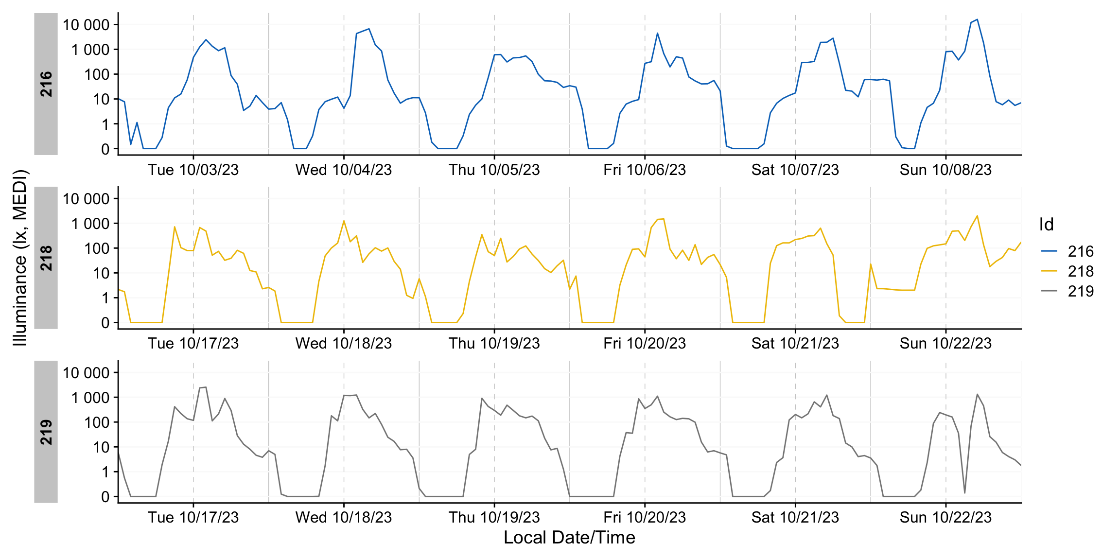
aggregate_Datetime() is a general‑purpose resampling utility that bins observations into fixed‑duration intervals and computes a summary statistic per bin. It is intentionally opinionated, providing sensible defaults (e.g., mean for numeric columns and mode for character/factor columns), but all summaries are configurable and additional metrics can be requested. Use it as a lightweight formatter to change the effective measurement interval after the fact (e.g., re‑epoching from 10 s to 1 min).
  dataset |>
  aggregate_Datetime("1 hour") |> #try to set different units: "15 mins", "2 hours",...
  gg_days(aes_col = Id)
aggregate_Date()
aggregate_Date() is a companion function that collapses each group into a single 24‑hour profile, optionally re‑epoching the data in the process. It is well‑suited to very large datasets when you need an overview of the average day. It applies the same summarization rules as aggregate_Datetime() and is equally configurable to your requirements:
dataset |>
  aggregate_Date(unit = "5 minutes") |>
  gg_days(aes_col = Id)
gg_doubleplot()
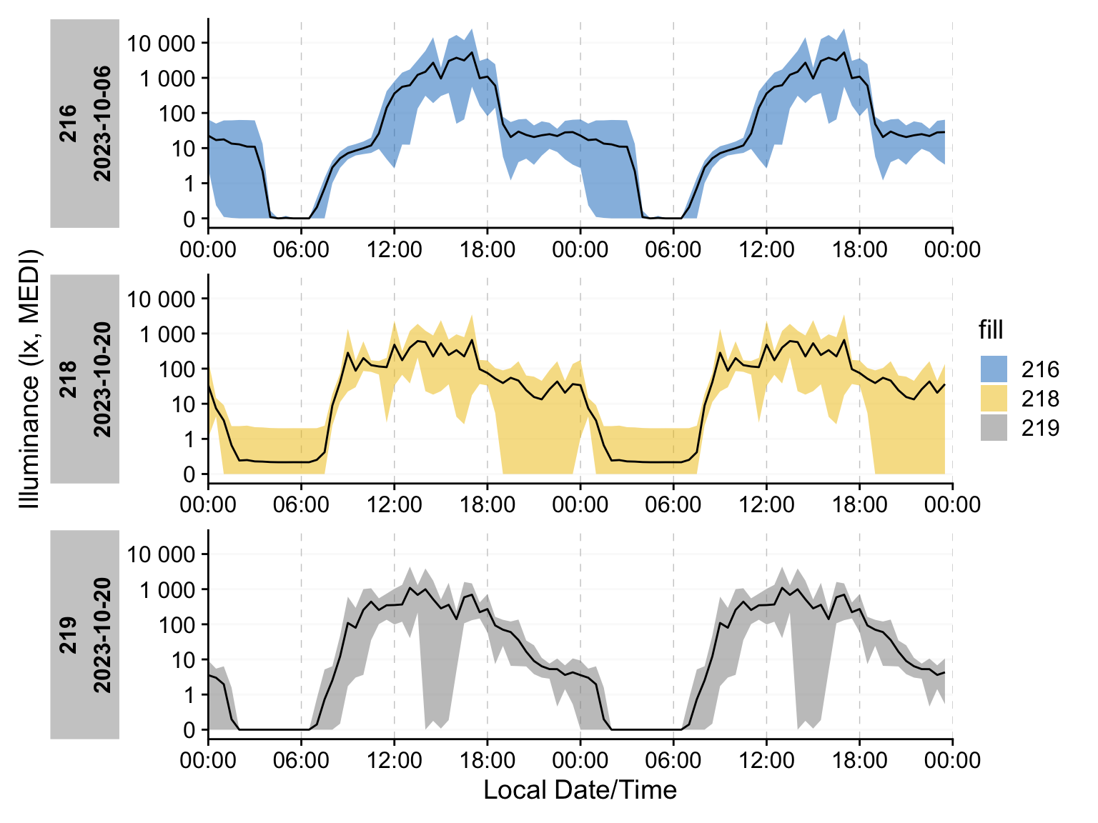
aggregate_Date() pairs well with gg_doubleplot(), which duplicates each day with an offset to reveal patterns that span midnight. While it can be applied to any dataset, use it on only a handful of days at a time to keep plots readable. If the dataset it is called on contains more than one day gg_doubleplot() defaults to displaying the next day instead of duplicating the same day.
dataset |>
  aggregate_Date(unit = "30 minutes") |>
  gg_doubleplot(aes_col = Id, aes_fill = Id)
# it is recommended to add photoperiod information after aggregating to the Date
# level and prior to the doubleplot for best results.
dataset |>
aggregate_Date(unit = "30 minutes") |>
add_photoperiod(coordinates, overwrite = TRUE) |>
gg_doubleplot(aes_fill = Id) |>
gg_photoperiod()Beyond inital variables
Both aggregate_Datetime() and aggregate_Date() allow for the calculation of additional metrics within their respective bins. One use case is to gauge the spread of the data within certain times. A simple approach is to plot the minimum and maximum value of a dataset that was condensed to a single day.
dataset |>
  aggregate_Date(unit = "30 minutes",
                 lower = min(MEDI), #create new variables...
                 upper = max(MEDI)  #...as many as needed
                 ) |>
  gg_doubleplot(geom = "blank") + # use gg_doubleplot only as a canvas
  geom_ribbon(aes(ymin = lower, ymax = upper, fill = Id), alpha = 0.5) +
  geom_line()
States
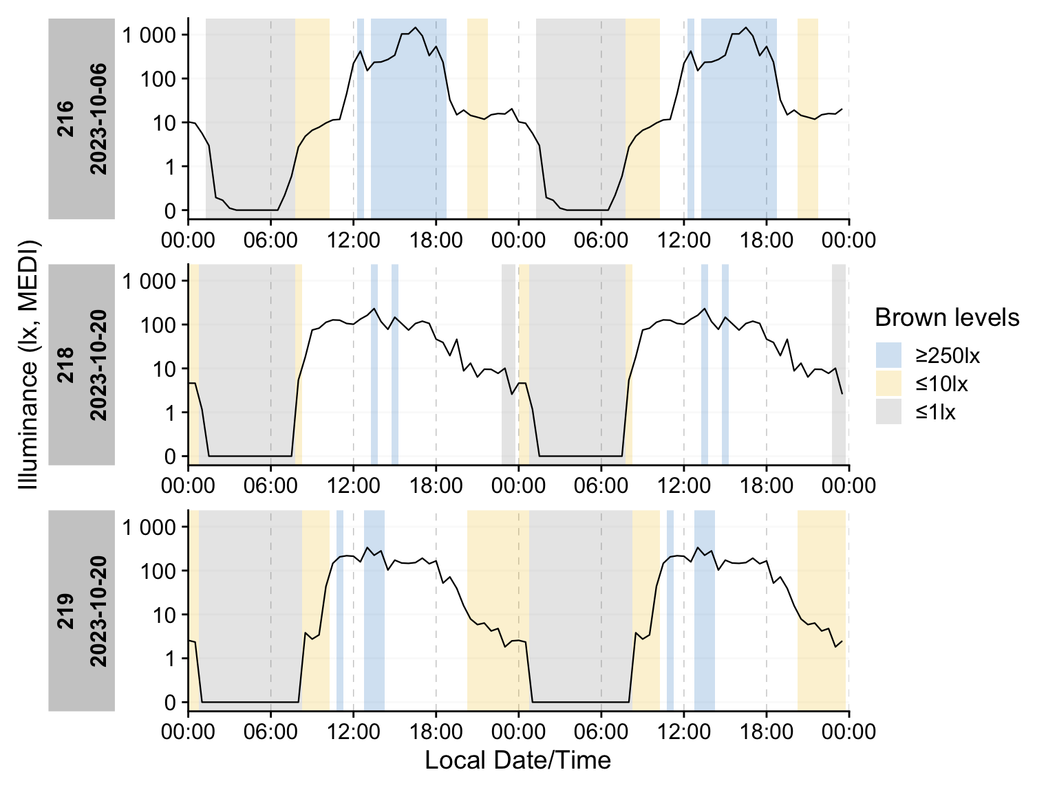
States, in the context of LightLogR, means any non-numeric variable. Those can be part of the dataset, be calculated from the dataset (e.g., mel EDI >= 250 lx), or added from an external source. We showcase some capabilities by dividing the dataset into sections by the Brown et al. (2022) recommendations for healthy lighting, using the Brown_cut() function.
dataset_1day <-
dataset |>
  Brown_cut() |> #creating a column with the cuts
  aggregate_Date(unit = "30 minutes",
                 numeric.handler = median #note that we switched from mean to median
                 ) |>
  mutate(state = state |> fct_relevel("≥250lx", "≤10lx", "≤1lx")) #order the levels
gg_state()
gg_state() augments an existing plot by adding background rectangles that mark state intervals. When multiple states are present, map them to distinct fills (or colors) to improve readability.
dataset_1day |>
  gg_doubleplot(col = "black", alpha = 1, geom = "line") |>
  gg_state(State.colname = state, aes_fill = state) +
  labs(fill = "Brown levels")
durations()
If you need a numeric summary of states, durations() computes the total time spent in each state per grouping (e.g., by Id, by day). With a small reshaping step, you can produce a tidy table showing the average duration each participant spends in each state:
dataset_1day |>
  group_by(state, .add = TRUE) |> #adding Brown states to the grouping
  durations(MEDI) |> #calculating durations
  ungroup() |>  #remove all grouping
  mutate(state = fct_na_value_to_level(state, "10-250lx")) |> #name NA level
  pivot_wider(id_cols = Id, names_from = state, values_from = duration) |> #reshape
gt()| Id | ≥250lx | ≤10lx | ≤1lx | 10-250lx |
|---|---|---|---|---|
| 216 | 21600s (~6 hours) | 14400s (~4 hours) | 23400s (~6.5 hours) | 27000s (~7.5 hours) |
| 218 | 10800s (~3 hours) | 5400s (~1.5 hours) | 28800s (~8 hours) | 48600s (~13.5 hours) |
| 219 | 7200s (~2 hours) | 23400s (~6.5 hours) | 27000s (~7.5 hours) | 28800s (~8 hours) |
extract_states() & summarize_numeric()
If your interest in states centers on individual occurrences - for example, how often a state occurred, how long each episode persisted, or when episodes began - use the following tools. extract_states() returns an occurrence‑level table (one row per episode) with start/end times and durations; summarize_numeric() then aggregates those episodes into concise metrics (e.g., counts, total duration, mean/median episode length) by the grouping you specify.
dataset_1day |>
  extract_states(state) |>
  summarize_numeric() |>
gt()| state | mean_epoch | mean_start | mean_end | mean_duration | total_duration | episodes |
|---|---|---|---|---|---|---|
| 216 | ||||||
| ≥250lx | 1800 | 12:45:00 | 15:45:00 | 10800s (~3 hours) | 21600s (~6 hours) | 2 |
| ≤10lx | 1800 | 14:00:00 | 16:00:00 | 7200s (~2 hours) | 14400s (~4 hours) | 2 |
| ≤1lx | 1800 | 01:15:00 | 07:45:00 | 23400s (~6.5 hours) | 23400s (~6.5 hours) | 1 |
| NA | 1800 | 17:27:00 | 14:09:00 | 5400s (~1.5 hours) | 27000s (~7.5 hours) | 5 |
| 218 | ||||||
| ≥250lx | 1800 | 14:00:00 | 14:30:00 | 1800s (~30 minutes) | 3600s (~1 hours) | 2 |
| ≤10lx | 1800 | 15:45:00 | 04:30:00 | 2700s (~45 minutes) | 5400s (~1.5 hours) | 2 |
| ≤1lx | 1800 | 11:45:00 | 15:45:00 | 14400s (~4 hours) | 28800s (~8 hours) | 2 |
| NA | 1800 | 12:25:00 | 16:55:00 | 16200s (~4.5 hours) | 48600s (~13.5 hours) | 3 |
| 219 | ||||||
| ≥250lx | 1800 | 11:45:00 | 12:45:00 | 3600s (~1 hours) | 7200s (~2 hours) | 2 |
| ≤10lx | 1800 | 17:25:00 | 11:35:00 | 7800s (~2.17 hours) | 23400s (~6.5 hours) | 3 |
| ≤1lx | 1800 | 00:45:00 | 08:15:00 | 27000s (~7.5 hours) | 27000s (~7.5 hours) | 1 |
| NA | 1800 | 11:55:00 | 14:35:00 | 9600s (~2.67 hours) | 28800s (~8 hours) | 3 |
It’s a wrap
This concludes the first part of the LightLogR tutorial. We hope it has given you a nice introduction to the package and convinced you to try it out with your own data and in your local installation. For more on LightLogR, we recommend the documentation page. If you want to stay up to date with the development of the package, you can sign up to our LightLogR mailing list.
Footnotes
If you are new to the R language or want a great introduction to R for data science, we can recommend the free online book R for Data Science (second edition) by Hadley Wickham, Mine Cetinkaya-Rundel, and Garrett Grolemund.↩︎
melanopic equivalent daylight-illuminance, CIE S026:2018↩︎
Guidolin, C., Zauner, J., & Spitschan, M., (2025). Personal light exposure dataset for Tuebingen, Germany (Version 1.0.0) [Data set]. URL: https://github.com/MeLiDosProject/GuidolinEtAl_Dataset_2025. DOI: doi.org/10.5281/zenodo.16895188↩︎


