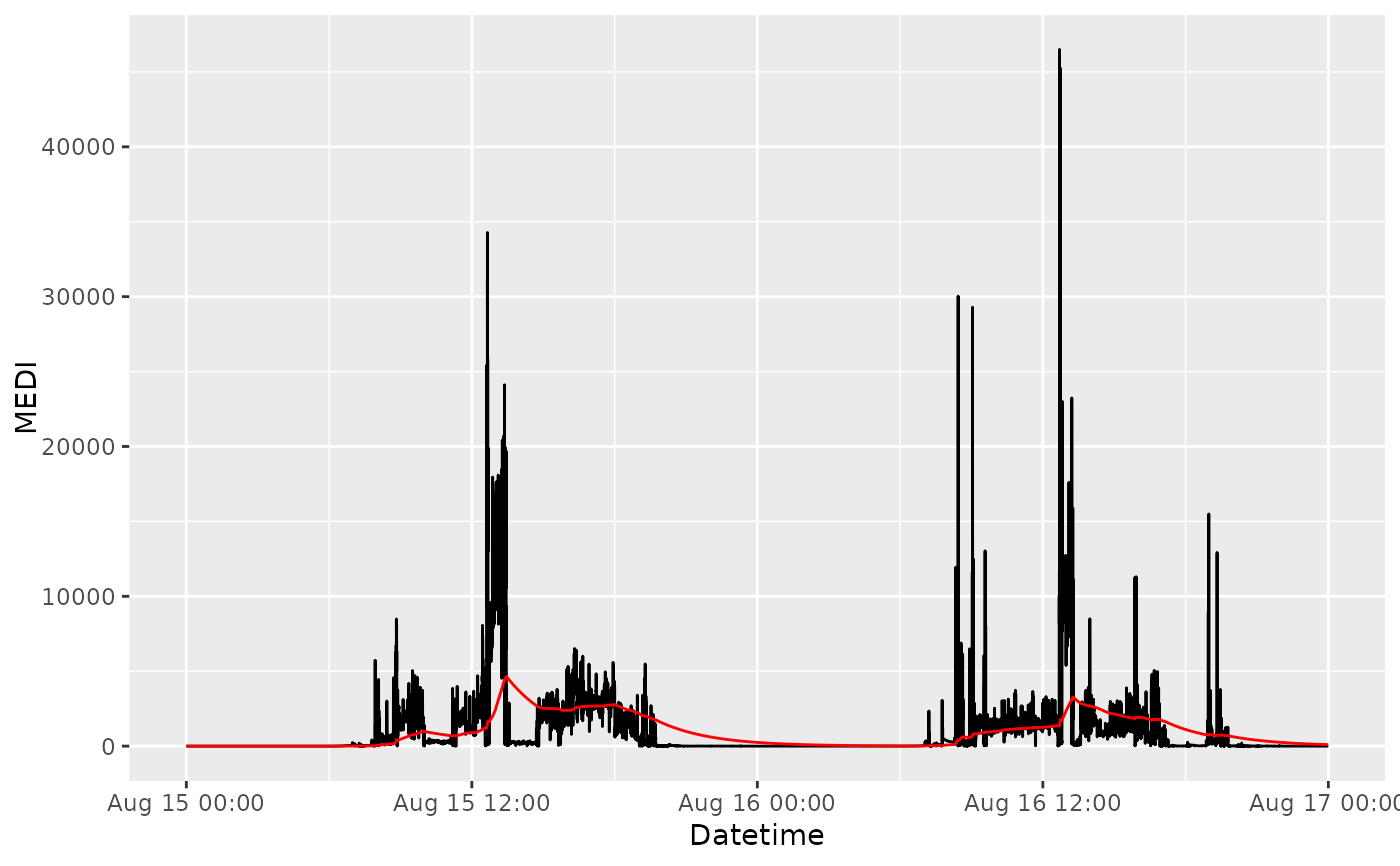
This function smoothes the data using an exponential moving average filter with a specified decay half-life.
Usage
exponential_moving_average(
  Light.vector,
  Time.vector,
  decay = "90 min",
  epoch = "dominant.epoch"
)
Arguments
- Light.vector
Numeric vector containing the light data. Missing values are replaced by 0.
- Time.vector
Vector containing the time data. Can be POSIXct, hms, duration, or difftime.
- decay
The decay half-life controlling the exponential smoothing. Can be either a duration or a string. If it is a string, it needs to be a valid duration string, e.g.,
"1 day"or"10 sec". The default is set to"90 mins"for a biologically relevant estimate (see the reference paper).- epoch
The epoch at which the data was sampled. Can be either a duration or a string. If it is a string, it needs to be either
"dominant.epoch"(the default) for a guess based on the data, or a valid duration string, e.g.,"1 day"or"10 sec".
Value
A numeric vector containing the smoothed light data. The output has the same
length as Light.vector.
Details
The timeseries is assumed to be regular. Missing values in the light data will be replaced by 0.
References
Price, L. L. A. (2014). On the Role of Exponential Smoothing in Circadian Dosimetry. Photochemistry and Photobiology, 90(5), 1184-1192. doi:10.1111/php.12282
Hartmeyer, S.L., Andersen, M. (2023). Towards a framework for light-dosimetry studies: Quantification metrics. Lighting Research & Technology. doi:10.1177/14771535231170500
See also
Other metrics:
bright_dark_period(),
centroidLE(),
disparity_index(),
dose(),
duration_above_threshold(),
frequency_crossing_threshold(),
interdaily_stability(),
intradaily_variability(),
midpointCE(),
nvRC(),
nvRD(),
nvRD_cumulative_response(),
period_above_threshold(),
pulses_above_threshold(),
threshold_for_duration(),
timing_above_threshold()
Examples
sample.data.environment.EMA = sample.data.environment %>%
  dplyr::filter(Id == "Participant") %>%
  filter_Datetime(length = lubridate::days(2)) %>%
  dplyr::mutate(MEDI.EMA = exponential_moving_average(MEDI, Datetime))

# Plot to compare results
sample.data.environment.EMA %>%
  ggplot2::ggplot(ggplot2::aes(x = Datetime)) +
  ggplot2::geom_line(ggplot2::aes(y = MEDI), colour = "black") +
  ggplot2::geom_line(ggplot2::aes(y = MEDI.EMA), colour = "red")

