Metrics • LightLogR

This article focuses on two important aspects of light logger analysis: structuring data into relevant groups and calculating personal light exposure metrics for them. LightLogR contains a large set of over 60 metrics and sub-metrics across multiple functions, where each constitutes a family of light exposure metrics. The following packages are needed for the analysis:

library(LightLogR)
library(tidyverse)
library(gt)
library(gtsummary)

Please note that this article uses the base pipe operator |>. You need an R version equal to or greater than 4.1.0 to use it. If you are using an older version, you can replace it with the magrittr pipe operator %>%.

Importing Data

We will use data imported and cleaned already in the article Import & Cleaning.

#this assumes the data is in the cleaned_data folder in the working directory
data <- readRDS("cleaned_data/ll_data.rds")

As can be seen by using gg_overview(), the dataset contains 17 ids with one weeks worth of data each, and one to three participants per week.

data |> gg_overview()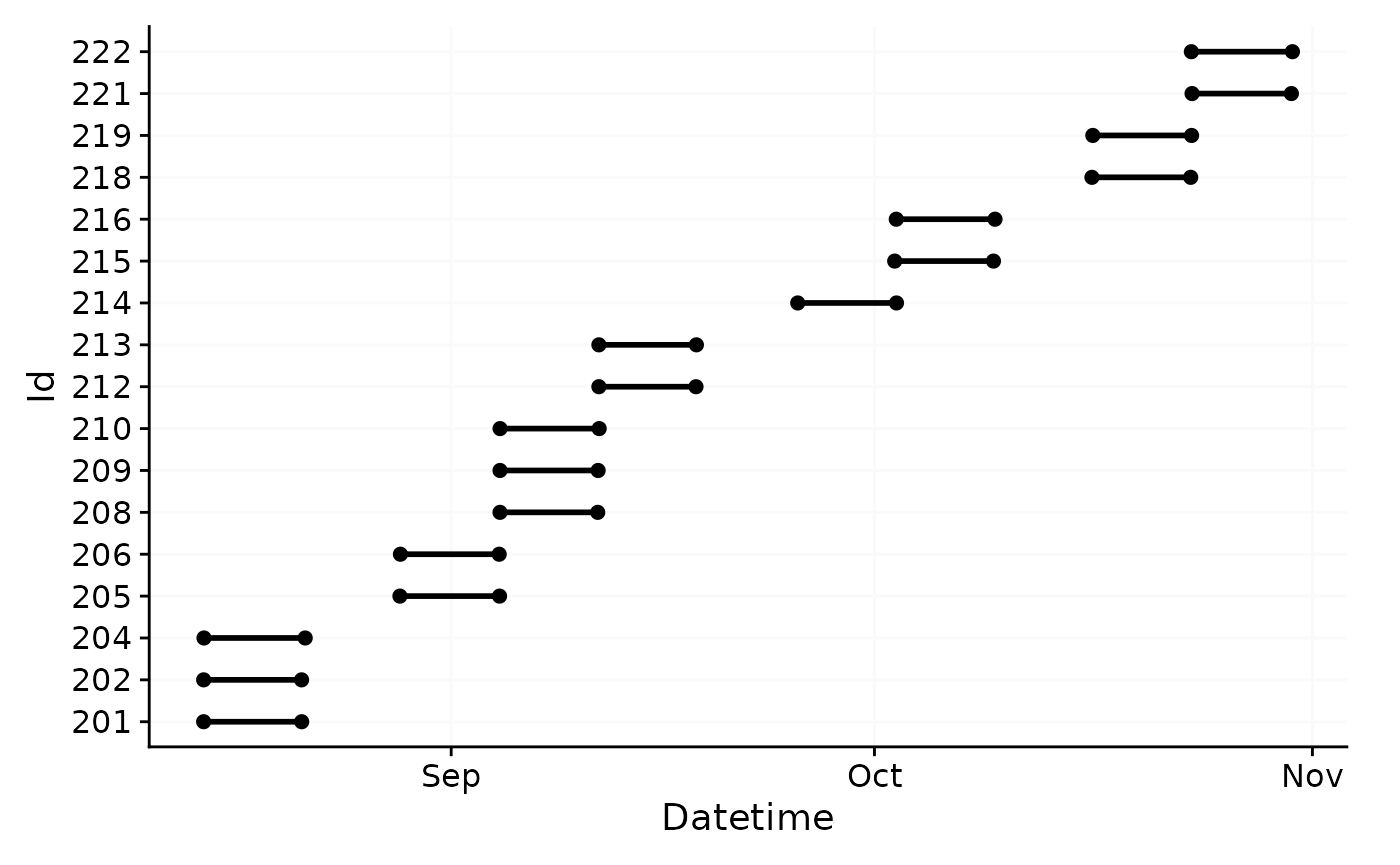

Metric principles

There are a lot of metrics associated with personal light exposure. You can find the function reference to all of them in the appropriate reference section. There are a few important distinctions between metrics that are important to understand:

Some metrics require or work best with a specific time frame, usually one day, while others are calculated over an arbitrary length of time. For example, the function interdaily_stability() calculates a metric over multiple days, while a function like midpointCE() calculates the midpoint of the cumulative light exposure within the given time series - this is less useful for multiple days, where the midpoint is just a time point during these days. E.g., for two similar light exposure patterns across two days, the midpoint of cumulative light exposure across those two days will be around midnight, which is not particularly informative. Much more sensible is the midpoint of the light exposure for each day. To enable this, data has to be grouped within days (or other relevant time frames, like sleep/wake-phase).
Some metrics are submetrics within a family and have to be actively chosen through the arguments of the function. An example is duration_above_threshold() that, despite its name also provides the metrics duration below threshold and duration within threshold. Depending on its comparison argument, and whether one or two thresholds are provided, the function will calculate different metrics.
Some metric functions calculate multiple submetrics at once, like bright_dark_period(). As stated above, this type of function contains metrics accessible through a function argument, period in this case, which allows to specify whether the brightest or darkest periods of the day are required. Independent of this, the function will calculate multiple submetrics at once, which are the onset, midpoint, and offset of the respective period, and also the mean light level during that period.

We will cover the practical considerations following from these aspects in the following sections. Further, every function documentation explicitly states whether different metrics are accessible through parameters, and which metrics are calculated by default.

Note: Most metrics require complete and regular data for a sensible output. While some metrics can handle missing data, it is generally advisable to clean the data before calculating metrics. LightLogR helps to identify gaps and irregularities and can also aggregate data to larger intervals, which can be acceptable for small gaps. In cases of larger gaps, dates or participants might have to be removed from analysis.

Metric calculation: basics

All metric functions are by default agnostic to the type of data. They require vectors of numeric data (e.g., light data) and commonly also of datetimes. This means that the functions can be used outside of the LightLogR framework, if applied correctly. Let us try this with a simple example for a days worth of light data for one participant across two functions.

data_Id201 <- 
  data |> 
    filter(Id == 201 & date(Datetime) == "2023-08-15")

data_Id201 |> 
  gg_day()

Time above threshold (TAT)

The first example metric we will calculate is the time above threshold (or TAT) for a threshold of 250 lx mel EDI. TAT is calculated by the function duration_above_threshold().

duration_above_threshold(
  Light.vector = data_Id201$MEDI,
  Time.vector = data_Id201$Datetime,
  threshold = 250
)
#> [1] "34500s (~9.58 hours)"

Specifying the argument comparison = "below" will calculate the time below the threshold.

duration_above_threshold(
  Light.vector = data_Id201$MEDI,
  Time.vector = data_Id201$Datetime,
  threshold = 250,
  comparison = "below"
)
#> [1] "51900s (~14.42 hours)"

And specifying two thresholds will calculate the time within the thresholds.

duration_above_threshold(
  Light.vector = data_Id201$MEDI,
  Time.vector = data_Id201$Datetime,
  threshold = c(10,250)
)
#> [1] "15320s (~4.26 hours)"

Brightest 10 hours of the day (L10)

The second example metric yields multiple submetrics at once. The function bright_dark_period() calculates the brightest and darkest periods of the day. By default, it calculates the brightest 10 hour period of the day. By setting as_df = TRUE, the function will return a data frame we can pipe to gt() for a nice output

bright_dark_period(
  Light.vector = data_Id201$MEDI,
  Time.vector = data_Id201$Datetime,
  as.df = TRUE
) |> 
  gt()

brightest_10h_mean	brightest_10h_midpoint	brightest_10h_onset	brightest_10h_offset
2506.202	2023-08-15 13:42:01	2023-08-15 08:42:11	2023-08-15 18:42:01

Looping

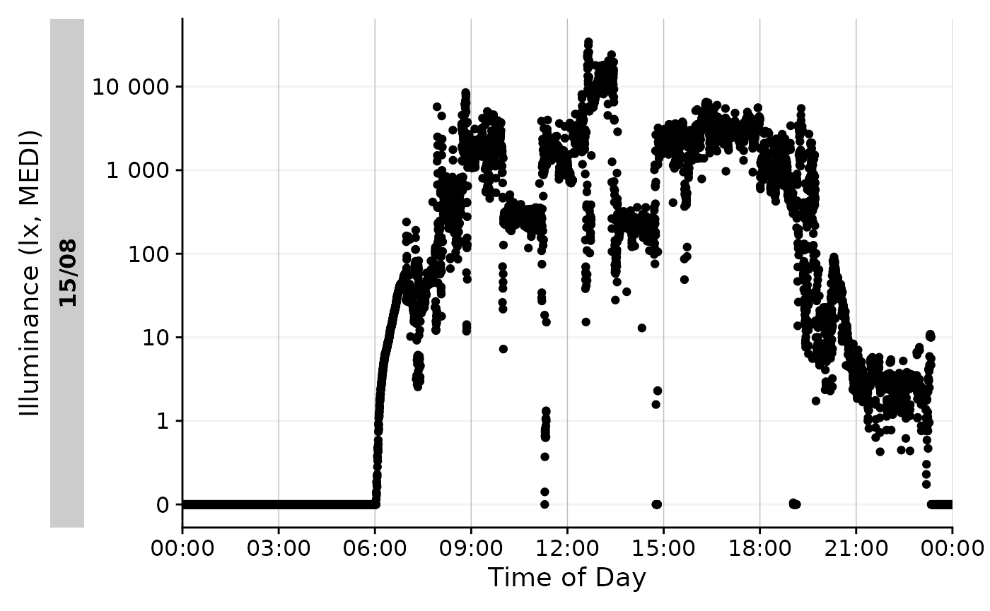
Calculating the darkest period of the day is tricky, as it likely traverses midnight. In the following code we can see that the darkest 10-hour period of day begins at midnight and ends at 10 am, which would be very coincidental. (Note that commonly, the darkest 5-hour period is calculated. We deviate from this to make this point.)

M10_wrong <- 
bright_dark_period(
  Light.vector = data_Id201$MEDI,
  Time.vector = data_Id201$Datetime,
  as.df = TRUE,
  period = "darkest",
  timespan = "10 hours"
)

M10_wrong |> gt()

darkest_10h_mean	darkest_10h_midpoint	darkest_10h_onset	darkest_10h_offset
305.2523	2023-08-15 04:59:51	2023-08-15 00:00:01	2023-08-15 09:59:51

We also see that this makes little sense, if we visualize this portion. The yellow color indicates the darkest 10-hour period of the day.

Onset <- M10_wrong$darkest_10h_onset
Offset <- M10_wrong$darkest_10h_offset

data_Id201 |> 
  gg_day(aes_col = Datetime >= Onset & Datetime <= Offset) +
  guides(color = "none")

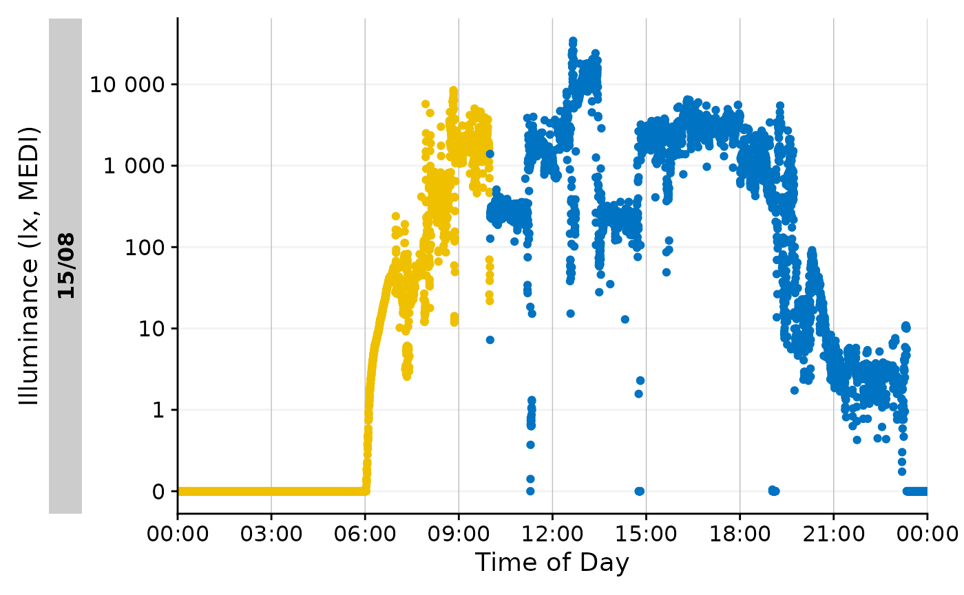
To solve this, bright_dark_period() and some other functions have the option to loop the day.

M10 <- 
bright_dark_period(
  Light.vector = data_Id201$MEDI,
  Time.vector = data_Id201$Datetime,
  as.df = TRUE,
  period = "darkest",
  timespan = "10 hours",
  loop = TRUE
)

M10 |> gt()

darkest_10h_mean	darkest_10h_midpoint	darkest_10h_onset	darkest_10h_offset
1.423622	2023-08-15 01:36:51	2023-08-15 20:37:01	2023-08-15 06:36:51

This is more plausible, and can also be visualized easily.

Onset <- M10$darkest_10h_onset
Offset <- M10$darkest_10h_offset

data_Id201 |> 
  gg_day(aes_col = Datetime >= Onset | Datetime <= Offset) +
  guides(color = "none")

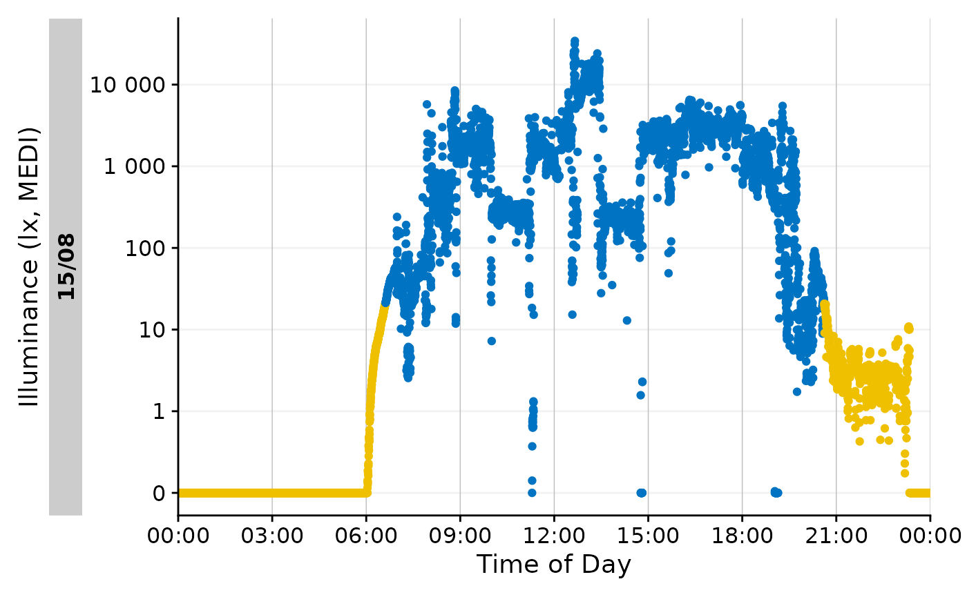
Metric calculation: advanced

More often than not, metrics are calculated for many participants over prolonged periods of time. In this case, the singular calculation as shown above is inefficient. The dplyr family of dplyr::summarize() and dplyr::reframe() make this much easier.

Preparation

As we only want to calculate metrics for days with full data, we will exclude Mondays from the data set.

data <- 
  data |> 
  dplyr::filter(weekdays(Datetime) != "Monday")

Summarize

The dplyr::summarize() function is used to calculate metrics for each group of data. In the following example, we will calculate Interdaily Stability (IS) for all participants in the data set, giving us the variability of the 24h light exposure patterns across the full 6 days of data compared to their average, ranging between 0 (Gaussian noise) and 1 (Perfect stability). For brevity, only the first 6 Ids will be shown.

data |> 
  summarize(
    IS = interdaily_stability(
      Light.vector = MEDI,
      Datetime.vector = Datetime
    )
  ) |> 
  head() |> 
  gt()

Id	IS
201	0.5263723
202	0.2058065
204	0.2759852
205	0.3332044
206	0.2453059
208	0.2007277

Grouping

By default, data imported with LightLogR is grouped by Id, which represents individual participants. When using the dplyr family of functions, grouping is essential, as it specifies the subgroups of data for which the metrics are calculated. In the following example, we will calculate the TAT 250 lx MEDI for all participants in the data set. We only show the first 6 participants, as it becomes readily apparent that time above threshold for 6 days might not be the most informative parametrization of the metric.

data |> 
  summarize(
    TAT_250 = duration_above_threshold(
      Light.vector = MEDI,
      Time.vector = Datetime,
      threshold = 250
    )
  ) |> 
  head() |> 
  gt()

Id	TAT_250
201	160180s (~1.85 days)
202	29970s (~8.32 hours)
204	147340s (~1.71 days)
205	98520s (~1.14 days)
206	6320s (~1.76 hours)
208	47140s (~13.09 hours)

Instead, we can calculate the TAT 250 lx MEDI for each participant and day of data. This is more informative, as it allows us to see how the metric changes over time. The final output is for the first two Ids.

#create a new column in the data set with the weekday
data$wDay <- wday(data$Datetime, label = TRUE, week_start = 1)

#group the data and calculate the metrics
TAT_250 <- 
data |> 
  group_by(wDay, .add = TRUE) |> 
  summarize(
    TAT_250 = duration_above_threshold(
      Light.vector = MEDI,
      Time.vector = Datetime,
      threshold = 250
    ), .groups = "drop_last"
  )

TAT_250 |> 
  head(12) |> 
  gt()

wDay	TAT_250
201
Tue	34500s (~9.58 hours)
Wed	32780s (~9.11 hours)
Thu	21820s (~6.06 hours)
Fri	31670s (~8.8 hours)
Sat	15010s (~4.17 hours)
Sun	24400s (~6.78 hours)
202
Tue	18760s (~5.21 hours)
Wed	6930s (~1.93 hours)
Thu	200s (~3.33 minutes)
Fri	200s (~3.33 minutes)
Sat	3130s (~52.17 minutes)
Sun	750s (~12.5 minutes)

Photoperiod

Another useful grouping factor is photoperiod, to differentiate the day into day and night. LightLogR contains a family of functions to easily deal with photoperiod. Here is a minimal example.

#specifying coordinates (latitude/longitude)
coordinates <- c(48.521637, 9.057645)

#adding photoperiod information
data <- 
  data |> 
  add_photoperiod(coordinates)

#calculating the metric
mean_Exposure <- 
data |> 
  group_by(photoperiod.state, .add = TRUE) |> 
  summarize(
    mean_MEDI = mean(MEDI), .groups = "drop_last"
  )

#showing the first three participants
mean_Exposure |> 
  head(6) |> 
  gt() |> 
  fmt_number(mean_MEDI)

photoperiod.state	mean_MEDI
201
day	962.52
night	0.70
202
day	317.06
night	2.28
204
day	2,194.02
night	6.94

This easily gives us metrics based on daily photoperiod. Metric calculation can utilize photoperiod information in other ways, too. More information on dealing with photoperiods can be found in the article Photoperiod.

Metric statistics

With the dataframe TAT_250, we can easily calculate statistics for each participant. This can be done manually, e.g., with another call to dplyr::summarize(), or semi-automatic, e.g., with packages like gtsummary. In the following example, we will calculate the mean and standard deviation of the TAT 250 lx MEDI for each participant, formatted as HH:MM through a styling function.

#styling formula for time
style_time <- function(x, format = "%H:%M"){
  x |> 
    as.numeric() |>  
    hms::as_hms() |> 
    as.POSIXlt() |> 
    format(format)
}

#Table output
TAT_250 |> 
  tbl_summary(by = Id, include = -wDay, 
              statistic = list(TAT_250 ~ "{mean} ({sd})"), 
              digits = list(TAT_250 ~ style_time),
              label = list(TAT_250 = "Time above 250 lx mel EDI")
              )

Characteristic	201 N = 6¹	202 N = 6¹	204 N = 6¹	205 N = 6¹	206 N = 6¹	208 N = 6¹	209 N = 6¹	210 N = 6¹	212 N = 6¹	213 N = 6¹	214 N = 6¹	215 N = 6¹	216 N = 6¹	218 N = 6¹	219 N = 6¹	221 N = 6¹	222 N = 6¹
Time above 250 lx mel EDI	07:24 (02:06)	01:23 (02:00)	06:49 (01:17)	04:33 (02:20)	00:17 (00:24)	02:10 (01:06)	04:07 (02:30)	08:39 (01:16)	04:50 (01:27)	02:33 (00:52)	04:38 (01:51)	02:06 (01:17)	04:07 (00:57)	01:26 (01:17)	02:45 (00:51)	01:00 (00:57)	00:33 (00:43)
¹ Mean (SD)

Metric calculation: batch

In the final section, we will add more metrics to the analysis, including ones with multiple sub-metrics. Further, we imagine we want to know how these metrics change from the first half of the experiment (August/September) to the second half (October/November). Finally, we will include a column Time.data in the data set, which will be used to calculate the metrics. This column format excludes the day information from the Datetime column, which avoids date-related issues when calculating the mean of the metrics. Finally, the unnest() call is used to flatten the table from the dataframe substructure that is created by MLIT250 and TAT250.

data <- data |> 
  mutate(
    Month = case_when(month(Datetime) %in% 8:9 ~ "Aug/Sep",
                      month(Datetime) %in% 10:11 ~ "Oct/Nov")
  ) |> 
  create_Timedata()

metrics <- 
  data |> 
  group_by(Month, Id, wDay) |> 
  summarize(
    MLIT250 = 
      timing_above_threshold(MEDI, Time.data, threshold = 250, as.df = TRUE),
    TAT250 = 
      duration_above_threshold(MEDI, Time.data, threshold = 250, as.df = TRUE),
    average_MEDI = 
      mean(MEDI),
    light_exposure = 
      sum(MEDI)/360, # 10 second epochs means 360 epochs in one hour. dividing by 360 gives the light exposure in lx·h
    .groups = "drop_last"
    ) |> 
  unnest(-Id)

#first 6 rows
metrics |> 
  head() |> 
  gt()

wDay	mean_timing_above_250	first_timing_above_250	last_timing_above_250	duration_above_250	average_MEDI	light_exposure
Aug/Sep - 201
Tue	13:55:49	07:48:01	19:43:41	34500s (~9.58 hours)	1094.7256	26273.415
Wed	12:53:04	07:03:01	19:46:41	32780s (~9.11 hours)	772.7199	18545.278
Thu	14:25:57	08:41:11	19:27:11	21820s (~6.06 hours)	263.1571	6315.771
Fri	13:12:42	07:14:41	18:51:21	31670s (~8.8 hours)	829.2784	19902.681
Sat	11:29:02	07:08:41	20:40:41	15010s (~4.17 hours)	559.5345	13428.829
Sun	12:46:28	07:23:01	19:12:21	24400s (~6.78 hours)	183.3234	4399.761

The operation above yields a data frame with six metrics across 102 participant days (6 days for 17 participants). The grouping for Month did not add additional groups, as each participant day is already solely in the "Aug/Sep" or "Oct/Nov" group. Next, we will regroup the data by Month and look at a summary table similar to the above, but for more metrics.

metrics <- 
  metrics |> 
  group_by(Month) |> 
  select(-Id, -wDay)

#Table output
metrics |> 
  tbl_summary(by = Month,
              statistic = list(all_continuous() ~ "{mean} (±{sd})"),
              digits = list(
                c(
                  mean_timing_above_250, first_timing_above_250, 
                  last_timing_above_250, duration_above_250
                  ) ~ style_time),
              label = list(
                mean_timing_above_250 = 
                  "mean timing above 250 lx mel EDI (HH:MM)",
                first_timing_above_250 = 
                  "first time above 250 lx mel EDI (HH:MM)",
                last_timing_above_250 = 
                  "last time above 250 lx mel EDI (HH:MM)",
                duration_above_250 = "duration above 250 lx mel EDI (HH:MM)",
                average_MEDI = "average mel EDI (lx)",
                light_exposure = "light exposure (lx·h)"
                )
              )

Characteristic	Aug/Sep N = 65¹	Oct/Nov N = 37¹
mean timing above 250 lx mel EDI (HH:MM)	13:39 (±01:43)	14:03 (±01:41)
first time above 250 lx mel EDI (HH:MM)	08:48 (±02:26)	10:14 (±02:20)
last time above 250 lx mel EDI (HH:MM)	19:09 (±02:20)	18:21 (±02:26)
duration above 250 lx mel EDI (HH:MM)	04:19 (±02:57)	02:02 (±01:32)
average mel EDI (lx)	535 (±505)	234 (±276)
light exposure (lx·h)	12,846 (±12,122)	5,618 (±6,612)
¹ Mean (±SD)

And that is all you need to work with metrics in LightLogR. Be sure to look at the documentation for each function to understand the parameters and outputs and at the reference section to get an overview of all available metrics.