Calculate photoperiod and boundary times

A family of functions to extract and add photoperiod information. photoperiod() creates a tibble with the calculated times of dawn and dusk for the given location and date. The function is a convenience wrapper for suntools::crepuscule() to calculate the times of dawn and dusk. By default, civil dawn and dusk are calculated, but the function can be used to calculate other times by changing the solarDep parameter (e.g., 0 for sunrise/sunset, 12 for nautical, and 18 for astronomical).

Taking a light exposure dataset as input, extract_photoperiod() calculates the photoperiods and their boundary times for each unique day in the dataset, given a location and boundary condition (i.e., the solar depression angle). Basically, this is a convenience wrapper for photoperiod() that takes a light logger dataset and extracts unique dates and the time zone from the dataset.

add_photoperiod() adds photoperiod information to a light logger dataset. Beyond the photoperiod information, it will categorize the photoperiod.state as "day" or "night". If overwrite is set to TRUE, the function will overwrite any columns with the same name.

solar_noon() calculates the solar noon for a given location and date. The function is a convenience wrapper for suntools::solarnoon(). The function has no companions like extract_photoperiod() or add_photoperiod(), but will be extended, if there is sufficient interest.

Usage

photoperiod(coordinates, dates, tz, solarDep = 6)

extract_photoperiod(
  dataset,
  coordinates,
  Datetime.colname = Datetime,
  solarDep = 6
)

add_photoperiod(
  dataset,
  coordinates,
  Datetime.colname = Datetime,
  solarDep = 6,
  overwrite = FALSE
)

solar_noon(coordinates, dates, tz)

Arguments

coordinates: A two element numeric vector representing the latitude and longitude of the location. Important note: Latitude is the first element and Longitude is the second element.
dates: A date of format Date, or coercible to Date through lubridate::as_date()
tz: Timezone of the data. Expects a character. You can look up the supported timezones with OlsonNames().
solarDep: A numerical value representing the solar depression angle between 90 and -90. This means a value of 6 equals -6 degrees above the horizon. Default is 6, equalling Civil dawn/dusk. Other common values are 12 degrees for Nautical dawn/dusk, 18 degrees for Astronomical dawn/dusk, and 0 degrees for Sunrise/Sunset. Note that the output columns will always be named dawn and dusk, regardless of the solarDep value.
dataset: A light logger dataset. Expects a dataframe. If not imported by LightLogR, take care to choose a sensible variable for the Datetime.colname.
Datetime.colname: column name that contains the datetime. Defaults to "Datetime" which is automatically correct for data imported with LightLogR. Expects a symbol. Needs to be part of the dataset. Must be of type POSIXct.
overwrite: Logical scalar. If TRUE, the function will overwrite any columns with the same name. If FALSE (default), the function will stop if any of the columns already exist in the dataset.

Value

photoperiod() returns a tibble with the calculated times of dawn and dusk for the given location and date, with the length equal to the dates input parameter . The tibble contains the following columns:

date with the date of the calculation, stored as class Date
tz with the timezone of the output, stored as class character
lat and lon with the latitude and longitude of the location, stored as class numeric
solar.angle with the negative solar depression angle, i.e. the sun elevation above the horizon. stored as class numeric
dawn and dusk with the calculated datetimes, stored as class POSIXct
photoperiod with the calculated photoperiod, stored as class difftime.

extract_photoperiod() returns a tibble of the same structure as photoperiod(), but with a length equal to the number of unique dates in the dataset.

add_photoperiod returns the input dataset with the added photoperiod information. The information is appended with the following columns: dawn, dusk, photoperiod, and photoperiod.state.

solar_noon() returns a tibble with the calculated solar noon

Details

Please note that all functions of the photoperiod family work with one coordinate pair at a time. If you have multiple locations (and multiple time zones), you need to run the function for each location separately. We suggest using a nested dataframe structure, and employ the purrr package to iterate over the locations.

Examples

 #example für Tübingen, Germany
 coordinates <- c(48.521637, 9.057645)
 dates <- c("2023-06-01", "2025-08-23")
 tz <- "Europe/Berlin"
 
 #civil dawn/dusk
 photoperiod(coordinates, dates, tz)
#>         date            tz      lat      lon solar.angle                dawn
#> 1 2023-06-01 Europe/Berlin 48.52164 9.057645          -6 2023-06-01 04:46:05
#> 2 2025-08-23 Europe/Berlin 48.52164 9.057645          -6 2025-08-23 05:55:03
#>                  dusk    photoperiod
#> 1 2023-06-01 21:57:43 17.19384 hours
#> 2 2025-08-23 20:56:37 15.02618 hours
 #sunrise/sunset
 photoperiod(coordinates, dates, tz, solarDep = 0)
#>         date            tz      lat      lon solar.angle                dawn
#> 1 2023-06-01 Europe/Berlin 48.52164 9.057645           0 2023-06-01 05:32:42
#> 2 2025-08-23 Europe/Berlin 48.52164 9.057645           0 2025-08-23 06:33:53
#>                  dusk    photoperiod
#> 1 2023-06-01 21:10:59 15.63821 hours
#> 2 2025-08-23 20:17:52 13.73304 hours
 #extract_photoperiod
 sample.data.environment |> 
   extract_photoperiod(coordinates)
#>         date            tz      lat      lon solar.angle                dawn
#> 1 2023-08-29 Europe/Berlin 48.52164 9.057645          -6 2023-08-29 06:03:20
#> 2 2023-08-30 Europe/Berlin 48.52164 9.057645          -6 2023-08-30 06:04:50
#> 3 2023-08-31 Europe/Berlin 48.52164 9.057645          -6 2023-08-31 06:06:20
#> 4 2023-09-01 Europe/Berlin 48.52164 9.057645          -6 2023-09-01 06:07:50
#> 5 2023-09-02 Europe/Berlin 48.52164 9.057645          -6 2023-09-02 06:09:19
#> 6 2023-09-03 Europe/Berlin 48.52164 9.057645          -6 2023-09-03 06:10:48
#>                  dusk    photoperiod
#> 1 2023-08-29 20:45:14 14.69838 hours
#> 2 2023-08-30 20:43:08 14.63828 hours
#> 3 2023-08-31 20:41:01 14.57813 hours
#> 4 2023-09-01 20:38:54 14.51793 hours
#> 5 2023-09-02 20:36:47 14.45769 hours
#> 6 2023-09-03 20:34:39 14.39742 hours


#add_photoperiod
added_photoperiod <-
 sample.data.environment |>
 add_photoperiod(coordinates)

added_photoperiod |> head()
#> # A tibble: 6 × 7
#> # Groups:   Id [1]
#>   Id          Datetime             MEDI dawn                dusk               
#>   <fct>       <dttm>              <dbl> <dttm>              <dttm>             
#> 1 Participant 2023-08-29 00:00:04     0 2023-08-29 06:03:20 2023-08-29 20:45:14
#> 2 Participant 2023-08-29 00:00:14     0 2023-08-29 06:03:20 2023-08-29 20:45:14
#> 3 Participant 2023-08-29 00:00:24     0 2023-08-29 06:03:20 2023-08-29 20:45:14
#> 4 Participant 2023-08-29 00:00:34     0 2023-08-29 06:03:20 2023-08-29 20:45:14
#> 5 Participant 2023-08-29 00:00:44     0 2023-08-29 06:03:20 2023-08-29 20:45:14
#> 6 Participant 2023-08-29 00:00:54     0 2023-08-29 06:03:20 2023-08-29 20:45:14
#> # ℹ 2 more variables: photoperiod <drtn>, photoperiod.state <chr>

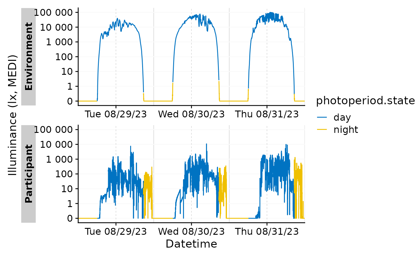
added_photoperiod |>
  filter_Date(length = "3 days") |>
  gg_days(aes_col = photoperiod.state,
          group = dplyr::consecutive_id(photoperiod.state),
          jco_color = TRUE
          )


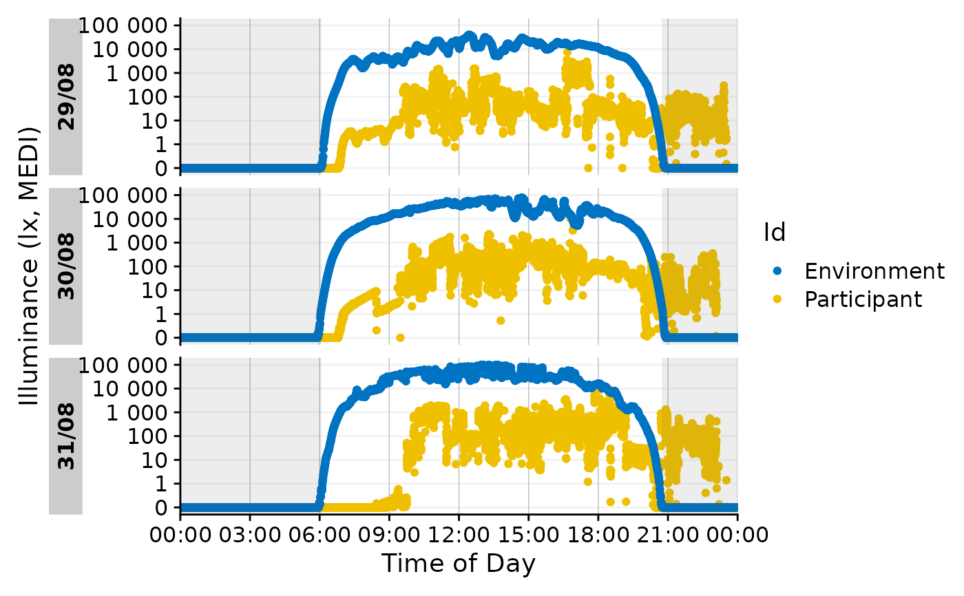
added_photoperiod |>
  filter_Date(length = "3 days") |>
  gg_day(aes_col = Id) +
  ggplot2:: geom_rect(
  data = \(x) x |> dplyr::ungroup(Id) |> dplyr::summarize(dawn = mean(dawn) |> hms::as_hms()),
  ggplot2::aes(xmin = 0, xmax = dawn, ymin = -Inf, ymax = Inf),
  alpha = 0.1
  ) +
  ggplot2:: geom_rect(
  data = \(x) x |> dplyr::ungroup(Id) |> dplyr::summarize(dusk = mean(dusk) |> hms::as_hms()),
  ggplot2::aes(xmin = dusk, xmax = 24*60*60, ymin = -Inf, ymax = Inf),
  alpha = 0.1
  )



 added_photoperiod |> dplyr::summarize(dawn = mean(dawn) |> hms::as_hms())
#> # A tibble: 2 × 2
#>   Id          dawn           
#>   <fct>       <time>         
#> 1 Environment 18:07:04.984169
#> 2 Participant 18:07:04.984169

 #solar_noon()
 solar_noon(coordinates, dates, tz)
#>         date            tz      lat      lon          solar.noon
#> 1 2023-06-01 Europe/Berlin 48.52164 9.057645 2023-06-01 13:21:35
#> 2 2025-08-23 Europe/Berlin 48.52164 9.057645 2025-08-23 13:26:21

Usage

Arguments

Value

Details

See also

Examples