Use case #01: A day in daylight

Open and reproducible analysis of light exposure and visual experience data (Advanced)

Author

Affiliation

Johannes Zauner

Technical University of Munich & Max Planck Institute for Biological Cybernetics, Germany

Last modified:

December 9, 2025

1 Preface

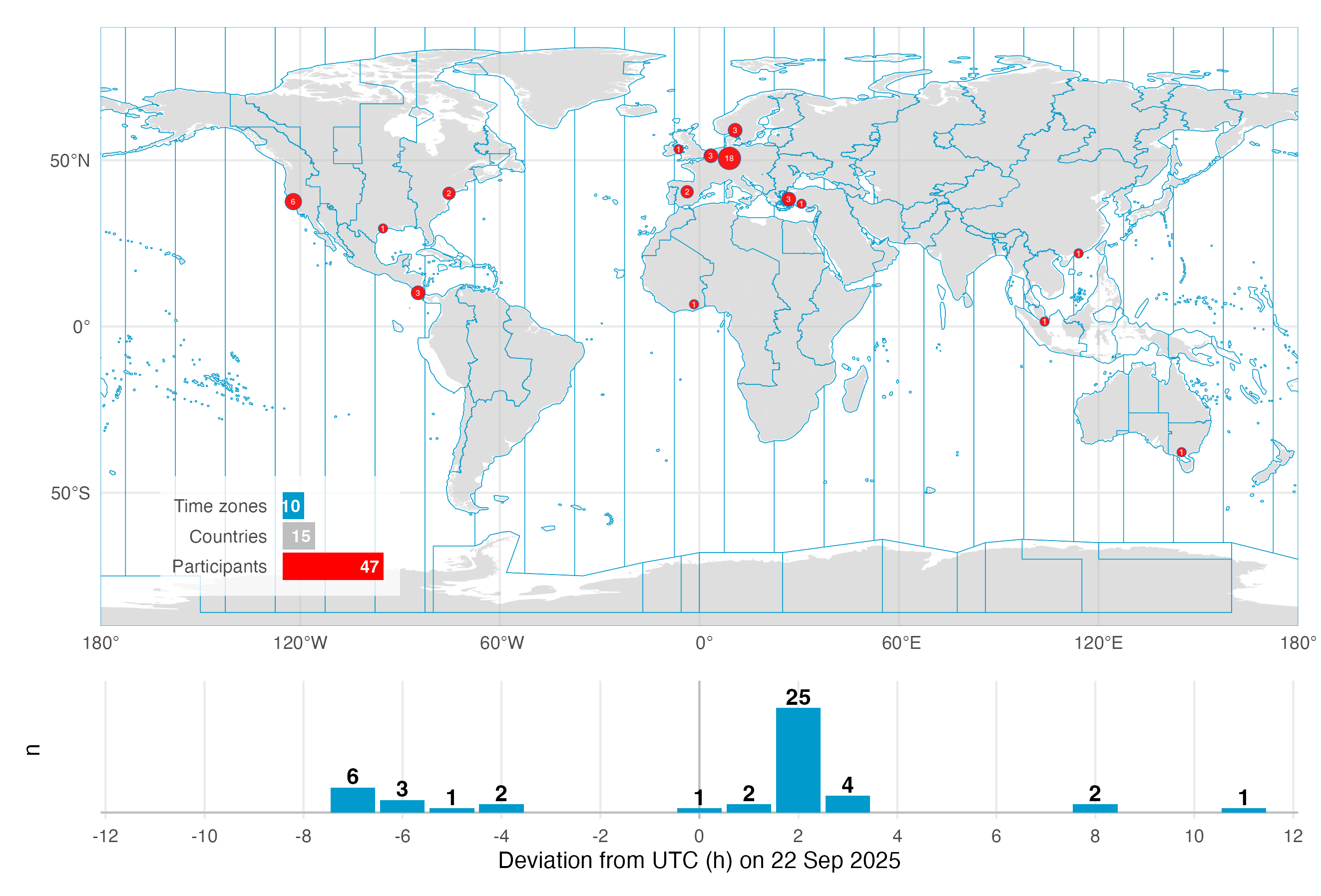
On the September 2025 equinox, over 50 participants across the globe logged and annotated their daily light exposure. While not a (traditional) study, the data is extraordinarily well suited to explore a diverse dataset across many participants in terms of geolocation, device-type, and contextual information, as participants logged their statechanges via a smartphone application. The dataset were analysed and presented as part of the A Day in Daylight event on 3 November 2025. They can be explored in an interactive dashboard. For this use case, we will take a subset of the datasets to explore workflows for these conditions, and summarize the data by combining it with activity logs and participant demographics.

For A Day in Daylight over 50 people across the globe logged and annotated their daily light exposure. 47 of those participants could be included in the analysis spanning many time zones. — For *A Day in Daylight* over 50 people across the globe logged and annotated their daily light exposure. 47 of those participants could be included in the analysis spanning many time zones.

The tutorial focuses on

setting up the import from multiple devices and time zones
handling multiple time zones once the data is imported
handling a large number of participants in a study
adding to and analysing participant-specific data (sex, age,…)

2 How this page works

This document contains the script for the online course series as a Quarto script, which can be executed on a local installation of R. Please ensure that all libraries are installed prior to running the script.

If you want to test LightLogR without installing R or the package, try the script version running webR, for a autonymous but slightly reduced version. These versions are indicated as (live), whereas the current version is considered (static), as it is pre-rendered.

To run this script, we recommend cloning or downloading the GitHub repository (link to Zip-file) and running the respective script. You will need to install the required packages. A quick way is to run:

renv::restore()

If this is your first course tutorial

This tutorial is considered as advanced. Basic functions in the LightLogR package as well as general tidy workflows are used without dedicated explanation. We recommend working through the beginner example if you are new to LightLogR (note that there is also a live variant).

3 Setup

We start by loading the necessary packages.

library(LightLogR) # main package
library(tidyverse) # for tidy data science
library(gt) # for great tables
library(ggridges) # for stacked plots within a panel
library(legendry) # for advanced plot axes
library(glue) # for easier label creation
library(zip) # to unzip files

4 Import

Note

Import works differently in this use case, because we import from different time zones and also devices. Would all devices be the same, or would the recordings have all happened in a single time zone, we would simply bulk import with import$device(files, tz)

4.1 Participant data

First, we collect a list of available data sets. Data are stored in a zip folder under data/a_day_in_daylight/lightloggers.zip.

path_light <- "data/a_day_in_daylight/lightloggers.zip"
files_light <- 
1  zip_list(path_light) |>
2  pull(filename) |>
3  tools::file_path_sans_ext()
files_light |> head()
4unzip(path_light, exdir = "data/a_day_in_daylight/lightloggers")

1: Collect a table of the files contained in the zip folder
2: Pull out the filenames from the table
3: remove file extenstions (.txt)
4: unzip all the files into the lightloggers subfolder

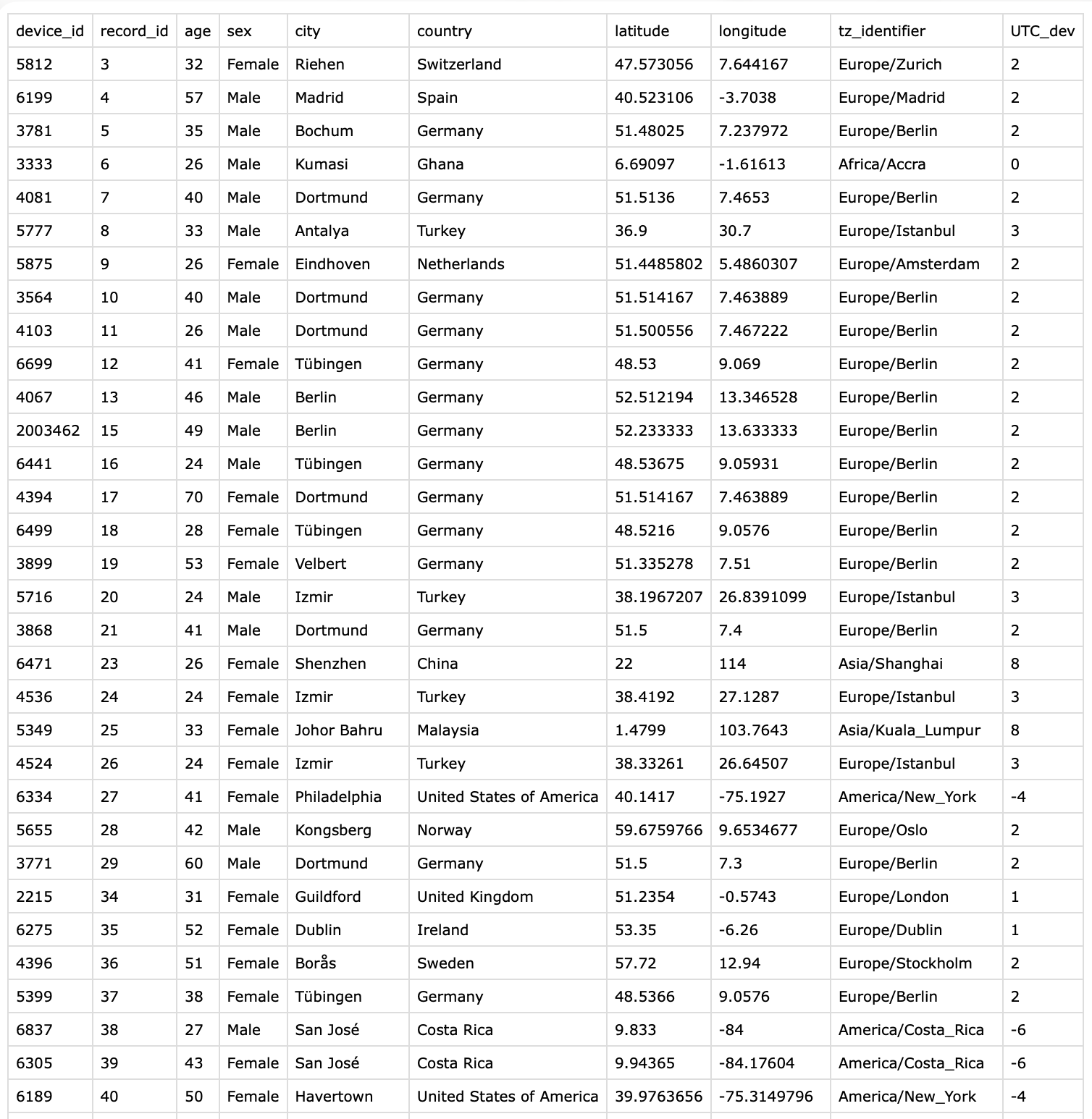
[1] "2003249" "2003462" "2215"    "3333"    "3564"    "3771"

Next we check which devices are declared in the participant metadata collected via a REDCap survey. We want to compare whether the device id’s from the file names match with the survey. Figure 1 shows the structure of the CSV file.

Figure 1: Excerpt from the participant data

participant_data <- read_csv("data/a_day_in_daylight/participant_metadata.csv")

1: Collect device id’s from survey
2: Check whether any entries are duplicated
3: Check whether all the files in the zip folder are represented in the survey

Rows: 47 Columns: 10
── Column specification ────────────────────────────────────────────────────────
Delimiter: ","
chr (4): sex, city, country, tz_identifier
dbl (6): device_id, record_id, age, latitude, longitude, UTC_dev

ℹ Use `spec()` to retrieve the full column specification for this data.
ℹ Specify the column types or set `show_col_types = FALSE` to quiet this message.

1survey_devices <- participant_data |> pull(device_id)
2survey_devices |> anyDuplicated()
3survey_devices |> setequal(files_light)

[1] 0
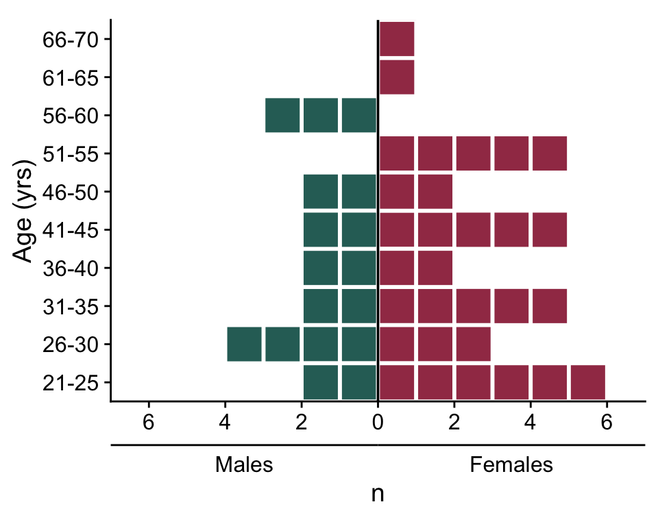
[1] TRUE

Before we import the wearable data, let’s make a plot of participants’ age(group) and sex.

4.2 Plot demographic data

First, we create a helper for the axis to indicate the sexes.

sex_lab <- primitive_bracket(
  key  = key_range_manual(
    start = c(-7,0), 
    end = c(0,7),
    name     = c("Males", "Females"),
    level = 1
  ),
  position = "bottom"
)

Then we create the actual plot:

participant_data |>  
  mutate(
1         age_group =
           cut(age,
               breaks = seq(20,70,5),
               labels = paste(4:13*5+1, 5:14*5, sep = "-"),
               right = TRUE,
               ordered_result = TRUE),
         ) |> 
2  summarize(n = n(), .by = c(sex, age_group)) |>
3  uncount(n) |>
  mutate(unit = row_number() - 0.5, 
         unit = if_else(sex == "Male", -unit, unit),
         .by = c(sex, age_group)) |>
4  mutate(n = ifelse(sex == "Male", -1, 1)) |>
  ggplot(aes(y= age_group, x = unit, fill = sex)) + 
  geom_tile(col = "white", lwd = 1) +
  geom_vline(xintercept = 0) +
  scale_x_continuous(breaks = seq(-6,6, by = 2), 
                     labels = c(6, 4, 2, 0, 2, 4, 6)) +
  scale_fill_manual(values = c(Male = "#2D6D66", Female = "#A23B54")) + 
  guides(fill = "none", alpha = "none",
         x = guide_axis_stack(
           "axis", sex_lab
         )) +
  cowplot::theme_cowplot() +
  coord_equal(xlim = c(-7, 7), expand = FALSE) +
  labs(y = "Age (yrs)", x = "n")

1: Convert age into age groups (length of five years)
2: Get the number of participants per age group and sex
3: Replicate each row n times
4: Change sign for males’ n

4.3 Import wearable data

Next, we import the light data. We do this inside participant_data. If you are not used to list columns inside dataframes, do not worry - we will take this one step at a time.

There are two devices in use: ActLumus and ActTrust. We need to import them separately, as they are using different file formats and thus import functions. In our case, device_id with four numbers indicates an ActLumus device, whereas seven numbers indicates an ActTrust. We add a column to the data indicating the Type of device in use. We also make sure that the spelling equals the supported_devices() list from LightLogR. Then we construct filename paths for all files.

all(c("ActLumus", "ActTrust") %in% supported_devices())

[1] TRUE

data <- 
participant_data |> 
  mutate(
    device_type = case_when(str_length(device_id) == 4 ~ "ActLumus",
                            str_length(device_id) == 7 ~ "ActTrust"
                            ),
    file_path = glue("data/a_day_in_daylight/lightloggers/{device_id}.txt")
    )
data |> 
  select(device_id, tz_identifier, device_type, file_path) |> 
  slice_head(n=5) |> 
  gt()

device_id	tz_identifier	device_type	file_path
5812	Europe/Zurich	ActLumus	data/a_day_in_daylight/lightloggers/5812.txt
6199	Europe/Madrid	ActLumus	data/a_day_in_daylight/lightloggers/6199.txt
3781	Europe/Berlin	ActLumus	data/a_day_in_daylight/lightloggers/3781.txt
3333	Africa/Accra	ActLumus	data/a_day_in_daylight/lightloggers/3333.txt
4081	Europe/Berlin	ActLumus	data/a_day_in_daylight/lightloggers/4081.txt

With this information we import our datasets into a column called light_data. Because this is going to be a list-column, we use the map family of functions from the {purrr} package, as they output a list for each input. Input, in our case, it the device_type, file_path, and tz_identifier in each row. Because the file names contain nothing but the Id, we don’t have to specify anything to the import function regarding Id, as the filename will be used by default.

data <- 
data |> 
  mutate(
    light_data = 
1      pmap(
2        list(x = device_type, y = file_path, z = tz_identifier),
3                       \(x, y, z) {
4                         import_Dataset(device = x,
                                        filename = y,
                                        tz = z,
                                        silent = TRUE)
                       }
    )
  )

1: pmap() takes a list of arguments, provides them row-by-row to a function, and outputs a list of results.
2: Inputs to our import function. In our case, because we are using the pmap() inside mutate, we can directly reference the dataset variables.
3: The function we want to be executed based on the inputs
4: LightLogR’s import function. We provide the arguments in the correct spot. Because we do not want to have 47 individual summaries and overview plots, we set the import to silent.

We end with one dataset per row entry. Let us have a look.

data$light_data[[1]] |> gg_days()

data$light_data[[20]] |> gg_days()

What about the import summary? We can still import the data the normal way (at least for one device type) - while they will all share the same time zone, it can still be used to get some initial insights about the data.

data |> 
1  filter(device_type == "ActLumus") |>
2  slice(-7, -32) |>
  pull(file_path) |> 
3  import$ActLumus() |>
4  invisible()

1: Select only participants with the ActLumus device
2: Remove two files that have a differing number of columns from the others. Likely, this is due to a software export setting. Importing those separately would not be an issue, just the mix is not possible.
3: Import function with standard settings
4: we are not interested in the actual data, just the side effect of the import summary.


Successfully read in 1'798'693 observations across 43 Ids from 43 ActLumus-file(s).
Timezone set is UTC.
The system timezone is Europe/Berlin. Please correct if necessary!

First Observation: 2025-09-03 12:54:25
Last Observation: 2025-09-29 15:37:15
Timespan: 26 days

Observation intervals: 
   Id    interval.time            n pct  
 1 2215  10s                  19128 100% 
 2 3333  10s                  19018 100% 
 3 3564  10s                  52401 100% 
 4 3771  10s                  52387 100% 
 5 3781  10s                  61946 100% 
 6 3852  10s                  79700 100% 
 7 3868  10s                  59500 100% 
 8 3899  10s                  54083 100% 
 9 3899  11s                      1 0%   
10 3899  133268s (~1.54 days)     1 0%   
# ℹ 51 more rows

5 Light data

5.1 Cleaning light data

In this section we will prepare the light data through the following steps:

resampling data to 5 minute intervals
filling in missing data with explicit gaps
removing data that does not fall between 2025-09-21 10:00:00 UTC and 2025-09-23 12:00:00 UTC, which contains all times where 22 September occurs somewhere on the planet
creating a local_time variable, which forces the UTC time zone on all time stamps. When we later merge all datasets, we will have Datetime to compare based on real-time measurements, and local_time to compare based on time of day.
adding photoperiod information to the data. It will use the local_time variable as a basis

data <-
  data |>
  mutate(
    light_data = 
      pmap(list(light_data, latitude, longitude), 
                  \(x, lat, lon) {
    x |>
1      aggregate_Datetime("5 mins") |>
2      gap_handler(full.days = TRUE) |>
      filter_Datetime(start = "2025-09-21 10:00:00", 
                      end = "2025-09-23 12:00:00", 
3                      tz = "UTC") |>
4      mutate(local_time = force_tz(Datetime, "UTC"), .before = Datetime) |>
5      add_photoperiod(c(lat, lon), overwrite = TRUE) |>
      mutate(across(c(dusk, dawn), \(x) force_tz(x, "UTC")))
  }))

1: Resample to 5 mins
2: Put in explicit gaps
3: Only leave a section of data
4: Adding a local_time colum
5: Adding photoperiod information and forcing it to the same time zone as local_time.

5.2 Visualizing light data

Now we can visualize the whole dataset - first by combining all datasets. There are two ways how to get to the complete dataset. First by joining only the wearable datasets:

1  join_datasets(!!!data$light_data)

1: The !!!data$light_data is basically equivalent to data$light_data[[1]], data$light_data[[2]],...

# A tibble: 28,128 × 41
# Groups:   Id [47]
   Id    local_time          Datetime            is.implicit EVENT TEMPERATURE
   <fct> <dttm>              <dttm>              <lgl>       <dbl>       <dbl>
 1 5812  2025-09-21 12:00:00 2025-09-21 12:00:00 FALSE           0        31.8
 2 5812  2025-09-21 12:05:00 2025-09-21 12:05:00 FALSE           0        32.0
 3 5812  2025-09-21 12:10:00 2025-09-21 12:10:00 FALSE           0        31.8
 4 5812  2025-09-21 12:15:00 2025-09-21 12:15:00 FALSE           0        31.5
 5 5812  2025-09-21 12:20:00 2025-09-21 12:20:00 FALSE           0        31.1
 6 5812  2025-09-21 12:25:00 2025-09-21 12:25:00 FALSE           0        30.8
 7 5812  2025-09-21 12:30:00 2025-09-21 12:30:00 FALSE           0        30.0
 8 5812  2025-09-21 12:35:00 2025-09-21 12:35:00 FALSE           0        29.3
 9 5812  2025-09-21 12:40:00 2025-09-21 12:40:00 FALSE           0        29.2
10 5812  2025-09-21 12:45:00 2025-09-21 12:45:00 FALSE           0        28.8
# ℹ 28,118 more rows
# ℹ 35 more variables: ORIENTATION <dbl>, PIM <dbl>, PIMn <dbl>, TAT <dbl>,
#   TATn <dbl>, ZCM <dbl>, ZCMn <dbl>, LIGHT <dbl>, IR.LIGHT <dbl>,
#   CAP_SENS_1 <dbl>, CAP_SENS_2 <dbl>, F1 <dbl>, F2 <dbl>, F3 <dbl>, F4 <dbl>,
#   F5 <dbl>, F6 <dbl>, F7 <dbl>, F8 <dbl>, MEDI <dbl>, CLEAR <dbl>,
#   STATE <dbl>, file.name <chr>, dawn <dttm>, dusk <dttm>, photoperiod <drtn>,
#   photoperiod.state <chr>, MS <dbl>, EXT.TEMPERATURE <dbl>, …

Or, and we use this method here, by unnesting the light_data in the data frame. While it requires a manual regrouping by Id, it has the added benefit, that all the participant data is kept with the wearable data.

light_data <- data |> unnest(light_data) |> group_by(Id)

Note

Note that we are working with two different devices, which export different variables, and also have different measurement qualities. In our specific case, both output a LIGHT variable that denotes photopic illuminance. We thus will use this variable to analyse light in this use case.

In a really study, however, mixing devices would have to be a far more deliberate step, and include some custom calibration.

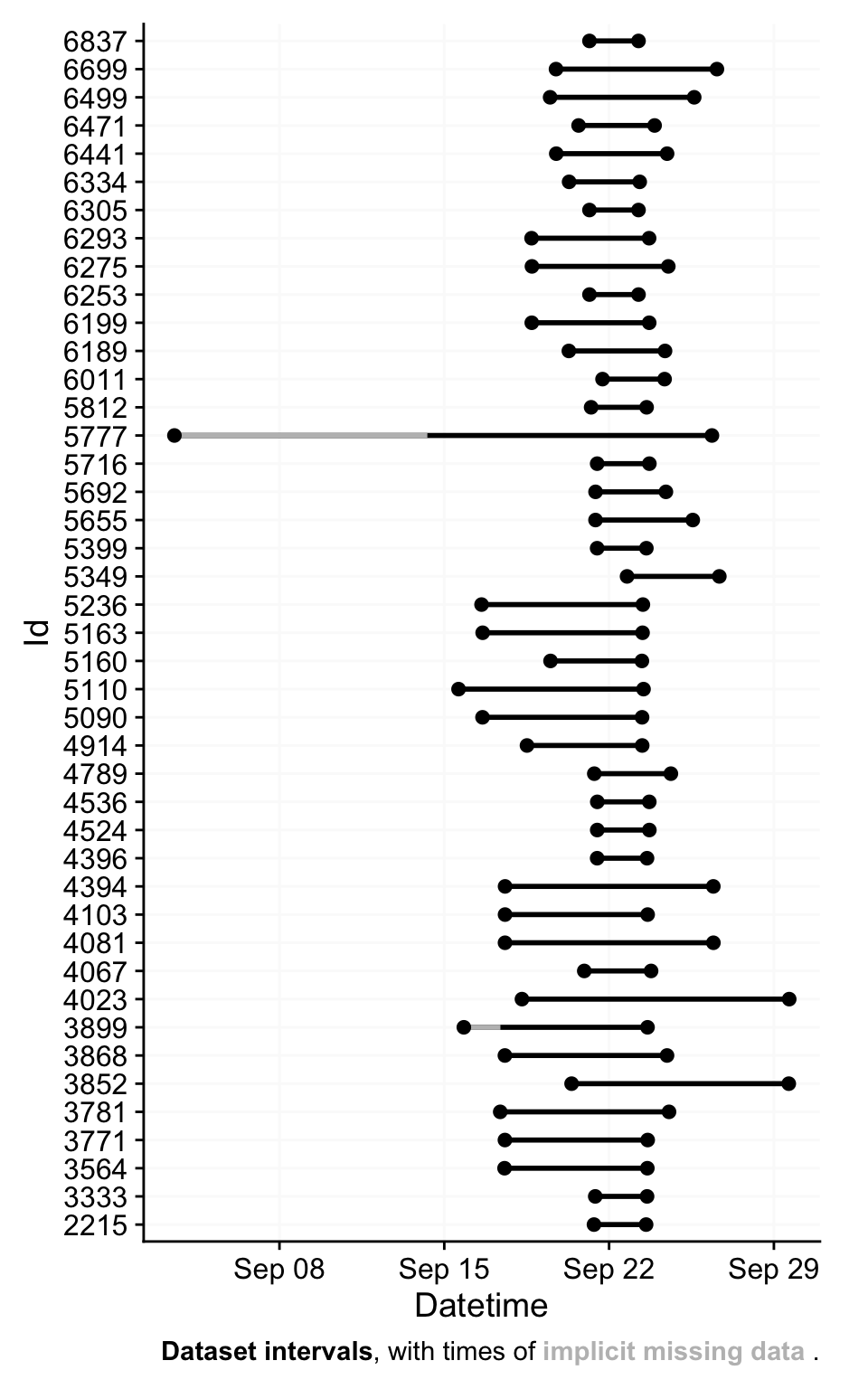
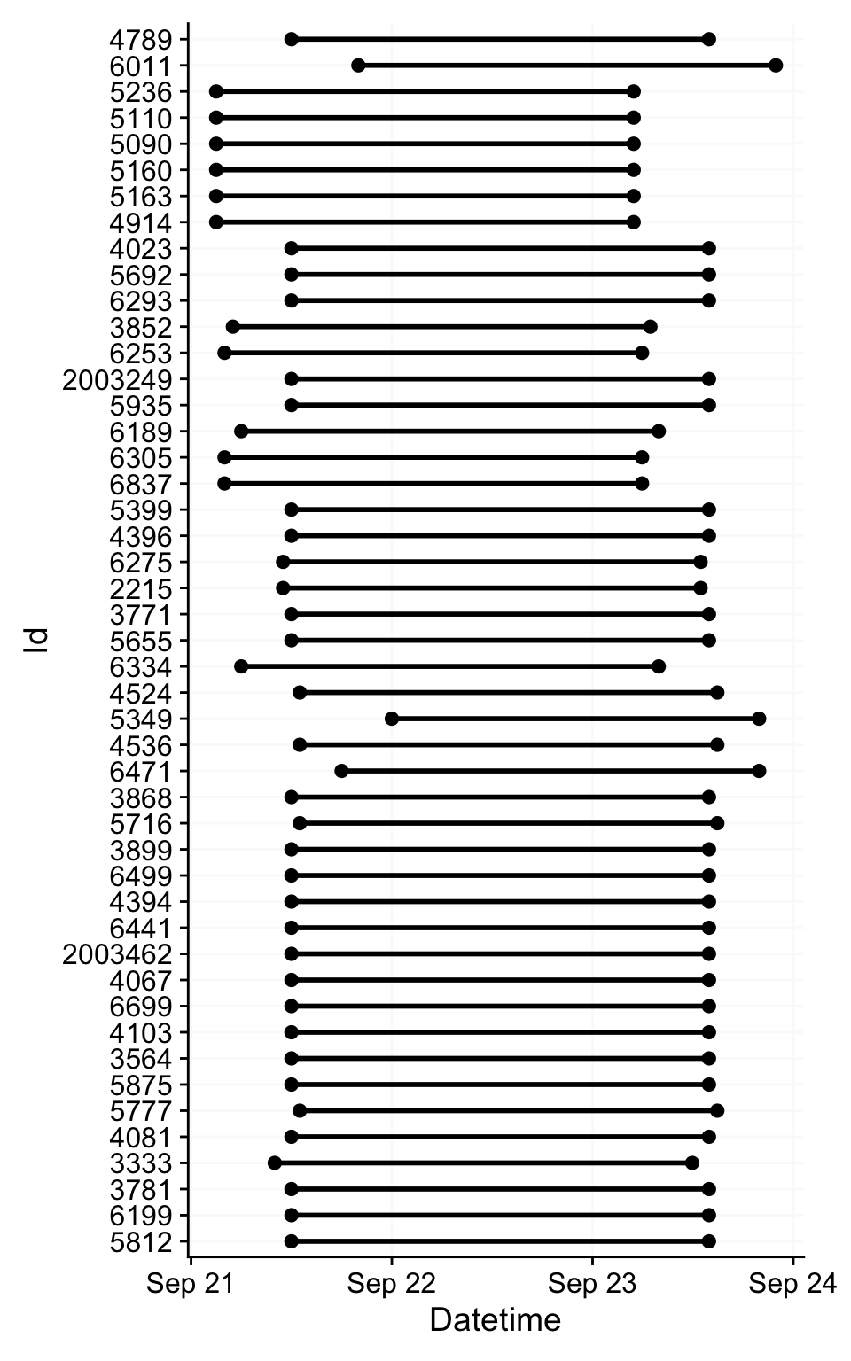
Here are some overviews of the data. With gg_overview():

light_data |> gg_overview(local_time)

With summary_overview():

light_data |> 
  summary_overview(LIGHT, Datetime.colname = local_time) |> 
  gt() |> 
  sub_missing()

name	mean	min	max
Participants	47.00000	—	—
Participant-days	141.00000	3.00000	3.000
Days ≥80% complete	46.00000	1.00000	1.000
Missing/Irregular	0.31000	0.31000	0.730
Photoperiod	13.16162	12.79672	13.708

And with summary_table()

light_data |> 
  summary_table(Variable.colname = LIGHT, 
                Datetime.colname = local_time,
                Variable.label = "Photopic illuminance (lx)",
                color = "red")

Warning: There were 42 warnings in `dplyr::summarize()`.
The first warning was:
ℹ In argument: `interdaily_stability(LIGHT, local_time, na.rm = TRUE, as.df =
  TRUE)`.
ℹ In group 4: `Id = 3333`.
Caused by warning in `interdaily_stability()`:
! One or more days in the data do not consist of 24 h.
Interdaily stability might not be meaningful for non-24 h days.
These days contain less than 24 h:
[1] "2025-09-21" "2025-09-22"
ℹ Run `dplyr::last_dplyr_warnings()` to see the 41 remaining warnings.

Overview
Summary table
TZ: UTC
Participants	Participants	47
Participant-days	Participant-days	141 (3 - 3)
Days ≥80% complete	Days ≥80% complete	46 (1 - 1)
Missing/irregular	Missing/Irregular	31.0% (31.0% - 73.0%)
Photoperiod	Photoperiod	13h 9m (12h 47m - 13h 42m)	¹
Metrics²
Dose	D (lx·h)	17,788 ±18,470 (1,891 - 81,883)
Duration above 250 lx	TAT₂₅₀	5h 3m ±2h 47m (25m - 10h 40m)
Duration within 1-10 lx	TWT_1-10	1h 55m ±1h 22m (5m - 6h 35m)
Duration below 1 lx	TBT₁	8h 54m ±1h 41m (5h 5m - 13h 10m)
Period above 250 lx	PAT₂₅₀	1h 51m ±1h 28m (5m - 6h 15m)
Duration above 1000 lx	TAT₁₀₀₀	1h 54m ±1h 35m (0s - 5h 55m)
First timing above 250 lx	FLiT₂₅₀	10:36 ±03:52 (06:00 - 21:55)	¹
Mean timing above 250 lx	MLiT₂₅₀	12:17 ±02:53 (04:16 - 17:35)	¹
Last timing above 250 lx	LLiT₂₅₀	17:24 ±02:21 (11:25 - 23:20)	¹
Brightest 10h midpoint	M10_midpoint	13:03 ±02:08 (08:35 - 19:55)	¹
Darkest 5h midpoint	L5_midpoint	03:13 ±04:23 (00:05 - 23:30)	¹
Brightest 10h mean³	M10_mean (lx)	289.9 ±265.8 (15.1 - 1,155.8)
Darkest 5h mean³	L5_mean (lx)	0.0 ±0.0 (0.0 - 0.0)
Interdaily stability	IS	1.000 ±0.000 (1.000 - 1.000)
Intradaily variability	IV	1.311 ±0.568 (0.338 - 2.233)
values show: mean ±sd (min - max) and are all based on measurements of Photopic illuminance (lx)
¹ Histogram limits are set from 00:00 to 24:00
² Metrics are calculated on a by-participant-day basis (n=46) with the exception of IV and IS, which are calculated on a by-participant basis (n=47).
³ Values were log 10 transformed prior to averaging, with an offset of 0.1, and backtransformed afterwards

What are the timezones of our two datetime columns now? Let´s find out

light_data |> 
  ungroup() |>
  summarize(tz_Datetime = tz(Datetime),
            tz_local_time = tz(local_time)
            )

# A tibble: 1 × 2
  tz_Datetime   tz_local_time
  <chr>         <chr>        
1 Europe/Zurich UTC

Why is that? local_time can be expected, we set it ourselves above. But why is Datetime now converted to Europe/Zurich. Looking at the first row of the participant data, we see that this is the time zone of the first participant:

participant_data |> slice_head() |> pull(tz_identifier)

[1] "Europe/Zurich"

When merging multiple time zones, the first time zone will be the one all others are converted to. It helps to remember that the underlying data does not change! Time-zone settings merely change the representation of the time points, not their position in time. The same way that a bar of length 254 mm can be expressed as 10 inches, without it changing the length of the bar. But because the first time zone of the participant list is very arbitrary, we will convert it to UTC as well. Instead of force_tz(), which changes the underlying time point, we use with_tz(), which simply changes the representation. Note that this change is merely cosmetic, i.e., it influences what you see when looking at the data in R. All calculations with that variable would be the same either way.

light_data <- 
  light_data |> 
  mutate(Datetime = with_tz(Datetime, "UTC"))
#rechecking:
light_data |> 
  ungroup() |>
  summarize(tz_Datetime = tz(Datetime),
            tz_local_time = tz(local_time)
            )

# A tibble: 1 × 2
  tz_Datetime tz_local_time
  <chr>       <chr>        
1 UTC         UTC

Then we create border points for the period of interest - start and end points in real time, and in local time, respectively.

start_rt <- as.POSIXct("2025-09-21 10:00:00", tz = "UTC")
start_lt <- as.POSIXct("2025-09-22 00:00:00", tz = "UTC")
end_rt <- as.POSIXct("2025-09-23 12:00:00", tz = "UTC")
end_lt <- as.POSIXct("2025-09-23 00:00:00", tz = "UTC")

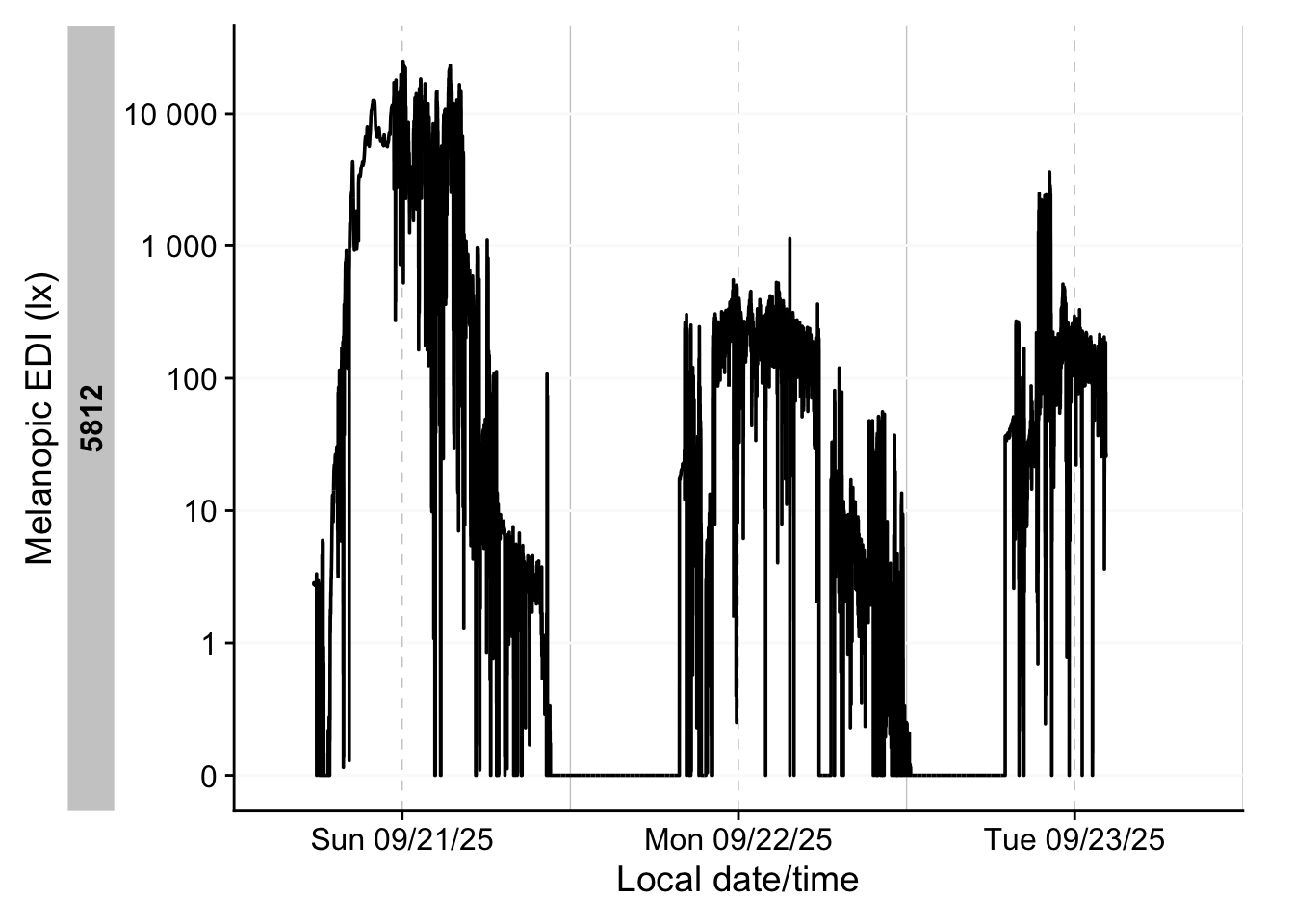
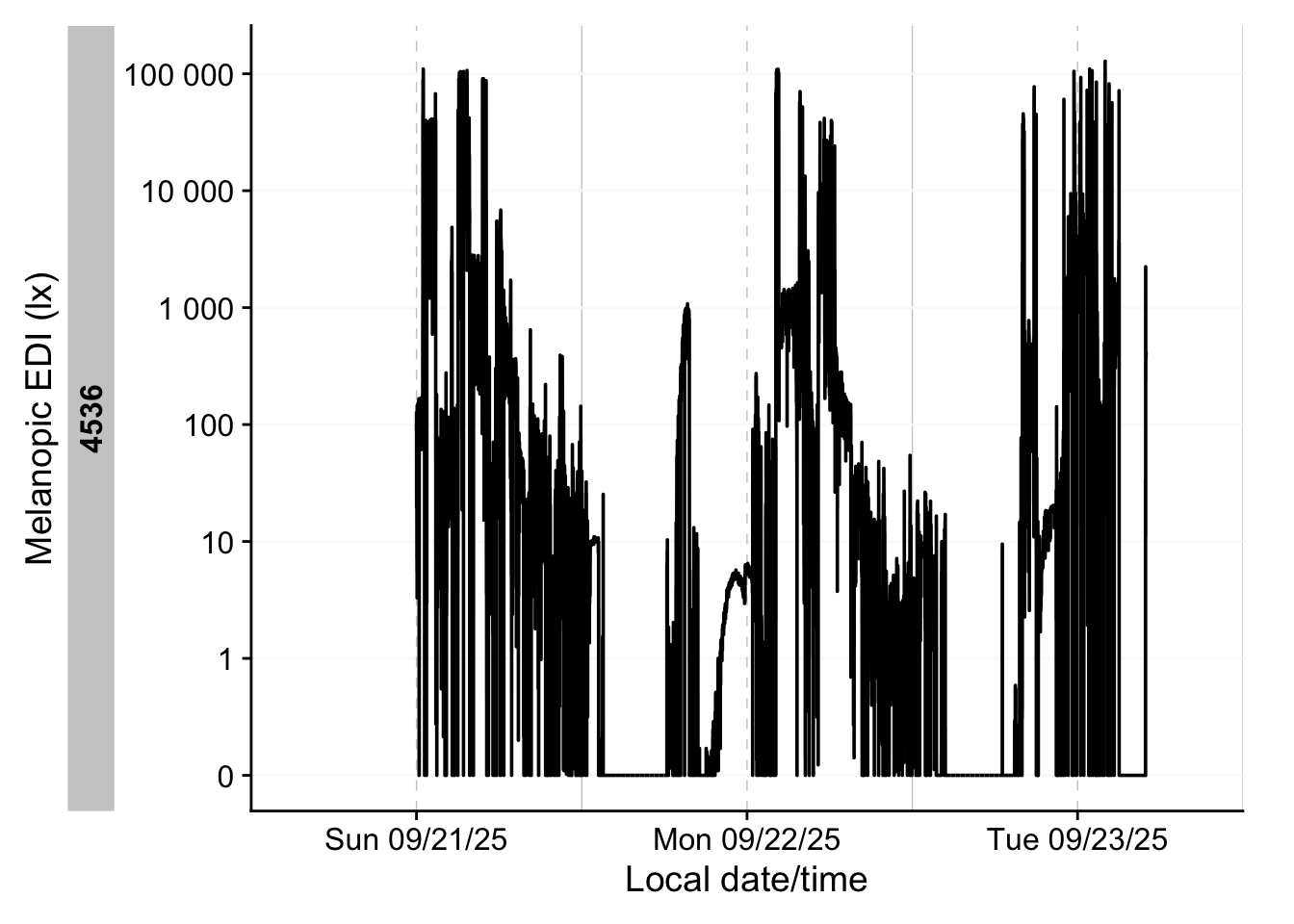
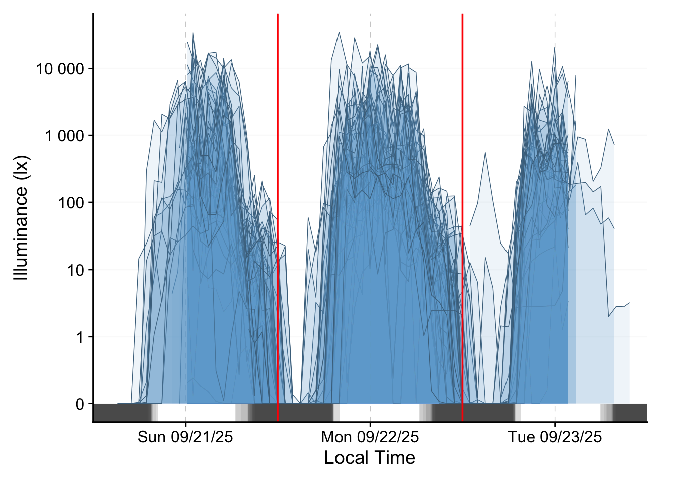
Then we plot all the datasets. Figure 2 shows how they relate in real time.

light_data |> 
  aggregate_Datetime("1hour") |> 
  gg_days(LIGHT,
          facetting = FALSE, 
          group = Id, 
          geom = "ribbon",
          lwd = 0.25,
          fill = "skyblue3",
          color = "skyblue4",
          alpha = 0.1,
          x.axis.label = "Real time",
          y.axis.label = "Illuminance (lx)"
          ) +
  geom_vline(xintercept = c(start_rt, end_rt), color = "red")

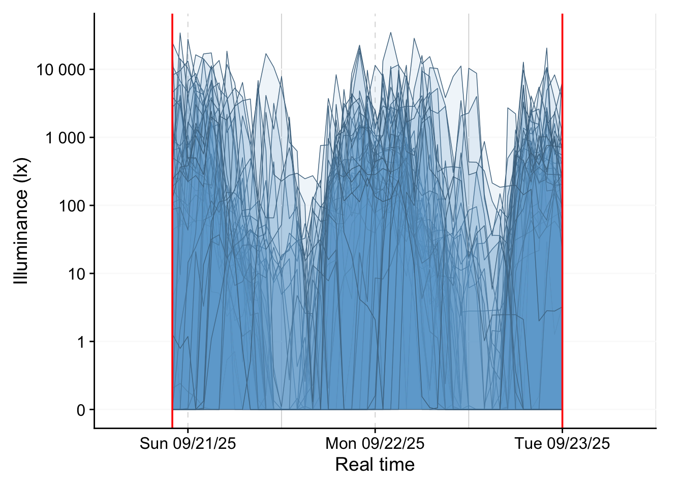
Figure 3 shows how they relate in local time, and also include a photoperiod indicator at the bottom.

light_data |> 
  aggregate_Datetime("1hour") |>
1  gg_days(LIGHT,
2          x.axis = local_time,
          geom = "ribbon",
          facetting = FALSE,
          fill = "skyblue3",
          color = "skyblue4",
          alpha = 0.1,
          group = Id, 
          lwd = 0.25,
          x.axis.label = "Local Time",
          y.axis.label = "Illuminance (lx)"
          ) |> 
3  gg_photoperiod(alpha = 0.1, Datetime.colname = local_time, ymax = 0) +
  geom_vline(xintercept = c(start_lt, end_lt), color = "red")

1: Replacing the default MEDI with our LIGHT variable that is available across all device types.
2: Setting the x.axis to the local_time
3: We also need to provide the deviating Datetime.colname for the photoperiods, otherwise the calculation of the average dusk and dawn by date will be erroneous.

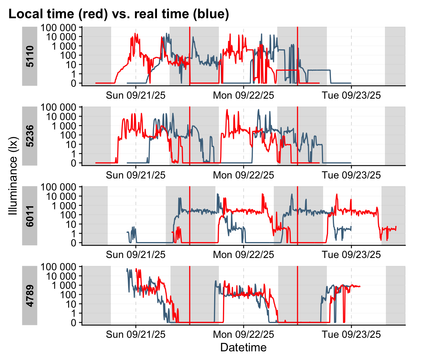
We can further create a small function that takes an indice and provide the realtime and localtime display of the dataset.

shift_plot <- function(group) {
light_data |> 
1  sample_groups(sample = group) |>
  gg_days(LIGHT,
          x.axis = Datetime,
          color = "skyblue4",
          group = Id, 
          x.axis.label = "Datetime",
          y.axis.label = "Illuminance (lx)"
          ) |> 
  gg_photoperiod(Datetime.colname = local_time) +
    geom_line(aes(x = local_time), col = "red") +
  geom_vline(xintercept = c(start_lt, end_lt), color = "red") +
    labs(title = "Local time (red) vs. real time (blue)")
}
shift_plot(44:47)

1: sample_groups() is a quick way to select groups

6 Time above threshold

In this section we calculate the time above threshold for the single day of 22 September 2025, depending on latitude and country. We require the local_time variable for that. Because we unnested the data into the participant data, that information is available to us.

TAT250 <- 
light_data |> 
1  filter_Date(start = "2025-09-22",
              length = "1 day",
              Datetime.colname = local_time) |>
  dplyr::summarize(
2    duration_above_threshold(
      LIGHT, local_time, threshold = 250, na.rm = TRUE,
      as.df = TRUE
    ),
3    latitude = first(latitude),
    longitude = first(longitude),
    country = first(country)
  ) |> 
4  mutate(n = n(), .by = country)

TAT250 |> head()

1: We reduce the length of the dataset
2: We calculate time above 250 lx
3: Extracting coordinates and country
4: Calculating how often a country is represented

# A tibble: 6 × 6
  Id    duration_above_250   latitude longitude country         n
  <fct> <Duration>              <dbl>     <dbl> <chr>       <int>
1 5812  22500s (~6.25 hours)    47.6       7.64 Switzerland     1
2 6199  31500s (~8.75 hours)    40.5      -3.70 Spain           2
3 3781  12000s (~3.33 hours)    51.5       7.24 Germany        17
4 3333  3000s (~50 minutes)      6.69     -1.62 Ghana           1
5 4081  21000s (~5.83 hours)    51.5       7.47 Germany        17
6 5777  27900s (~7.75 hours)    36.9      30.7  Turkey          4

We plot this information with a custom function, which lets us quickly exchange latitude and longitude.

TAT250_plot <- function(value){
TAT250 |> 
  ggplot(
    aes(
1      x= fct_reorder(Id, duration_above_250),
      y = duration_above_250))+
  geom_col(aes(fill = {{ value }})) +
  scale_fill_viridis_b(labels = \(x) paste0(x, "°"))+
2  scale_y_time(labels = style_time,
               expand = FALSE) + 
  theme_minimal() +
  theme_sub_axis_x(text = element_blank(), line = element_line()) +
  theme_sub_panel(grid.major.x = element_blank())+
  labs(x = "Participants", y = "Time above 250lx (HH:MM)")
}

3TAT250_plot(latitude) |> plotly::ggplotly()

1: Ordering the output by their time above 250lx
2: style_time() is a LightLogR convenience function that produces nice time labels
3: Making the plot interactive

Next we display the metric by country. Because the individual variance of these data is very high, we also choose to add information about the number of individuals within a country.

TAT250 |> 
  ggplot(
    aes(
      y= fct_reorder(country, duration_above_250), 
      x = duration_above_250))+
  geom_boxplot(aes(col = n)) +
  scale_color_viridis_b(breaks = c(1, 3, 5, 10, 15))+
  scale_x_time(labels = style_time) + 
  theme_minimal() +
  theme_sub_panel(grid.major.y = element_blank())+
  labs(y = NULL, x = "Time above 250lx (HH:MM)")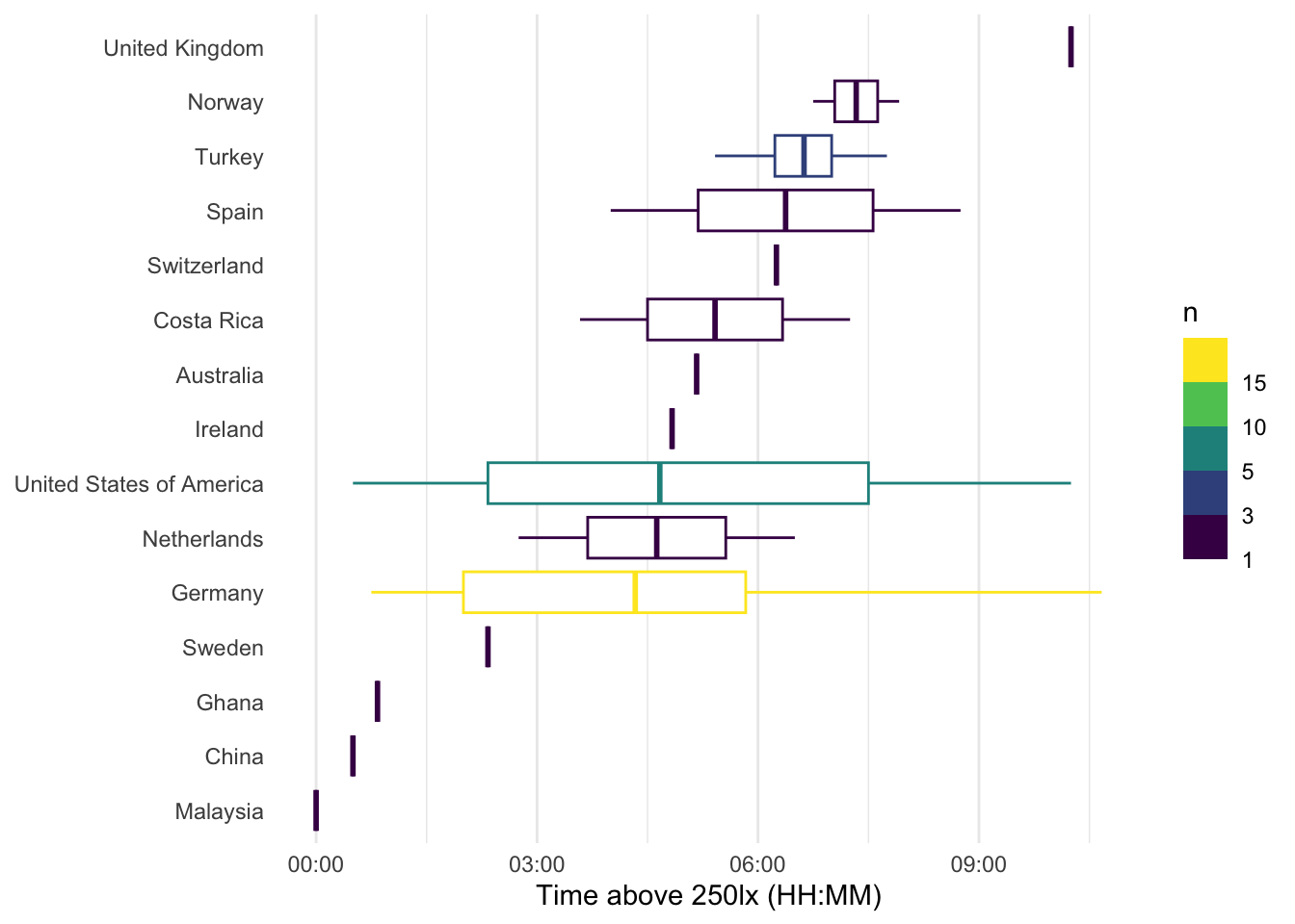

7 Event data

The last major aspect we will cover in this use case, are the activity logs that participants filled in, whenever their status changed - be it whether they took off their device, changed location, activity, or switched light settings. The activity logs are available as an R object here, this has the benefit that variable labels are retained.

On the order of including wear-information

In a regular analysis, we would use the non-wear information at hand before we calculated any metrics as we did in the prio sections. For this online course, however, we set the order of aspects also after didactic aspects. We want to close with this aspect here, as the activity logs are quite complex. Normally, the non-wear information would be added (and those times excluded) much earlier.

We start by loading in the logs and display a small portion:

load("data/a_day_in_daylight/events.RData")
dim(events)

[1] 1827   28

events |> slice_head(n = 5) |> gt()

Start Date	Record ID	Wear type: Are you wearing the light logger at the moment?	Are you alone or with others?	Wear/Non-wear context	Activity	Non-wear wearable position	Nightstand wearable measurement direction	What is your general context?	General setting	Indoor settings	Specific indoor setting	Indoors setting (home)	Indoors setting (work)	Indoors setting (health facility)	Indoors setting (learning facility)	setting_indoors_leisurespace	Indoors setting (retail facility)	Outdoor-Indoor mixed settings	Outdoor settings	Daylight conditions	Electric lighting conditions	Phone use	Tablet use	Computer use	Television use	Were the lighting conditions in this setting self-selected?
2025-09-21 11:59:36	3	Wear	With others	Moderate activity	Moderate activity	NA	NA	Outdoors	Leisure	NA	NA	NA	NA	NA	NA	NA	NA	NA	Leisure	Shade / cloudy	NA	FALSE	FALSE	FALSE	FALSE	NA
2025-09-21 13:16:29	3	Wear	With others	Light activity	Light activity	NA	NA	Mixed	Other	NA	NA	NA	NA	NA	NA	NA	NA	Other	NA	Shade / cloudy	NA	FALSE	FALSE	FALSE	FALSE	NA
2025-09-21 16:24:49	3	Wear	With others	Sedentary	Sedentary	NA	NA	Mixed	Transportation (car/taxi)	NA	NA	NA	NA	NA	NA	NA	NA	Transportation (car/taxi)	NA	NA	NA	FALSE	FALSE	FALSE	FALSE	NA
2025-09-21 17:20:15	3	Wear	With others	Light activity	Light activity	NA	NA	Mixed	Other	NA	NA	NA	NA	NA	NA	NA	NA	Other	NA	Shade / cloudy	NA	FALSE	FALSE	FALSE	FALSE	NA
2025-09-21 18:09:41	3	Wear	With others	Sedentary	Sedentary	NA	NA	Mixed	Transportation (car/taxi)	NA	NA	NA	NA	NA	NA	NA	NA	Transportation (car/taxi)	NA	Shade / cloudy	NA	FALSE	FALSE	FALSE	FALSE	NA

startdate marks the local time when an activity was logged. As per the instructions, it should be valid until the next activity is logged. This allows us to put start and end timepoints to each row.

events <-
  events |> 
  dplyr::mutate(
1    start = as.POSIXct(startdate, tz = "UTC"),
2    status.duration = c(diff(start), NA_real_),
3    end = case_when(
              is.na(lead(start)) ~ (start + dhours(6)),
              .default = start + status.duration
              ),
4    setting_light = case_when(type == "Bedtime" ~ "Bed",
                              type == "Non-wear" ~ "Non-wear",
                              .default = setting_light |> as.character()) |>
                    factor(levels =
                           c("Bed", "Indoors", "Mixed", "Outdoors", "Non-wear")
                           ),
5    record_id = as.numeric(record_id),
6    .by = record_id,
    .after = startdate) |> 
7  left_join(participant_data |> select(device_id, record_id), by = "record_id") |>
  rename(Id = device_id) |>
  mutate(Id = factor(Id)) |>
8  semi_join(participant_data, by = "record_id")

1: The start variable is already presend, but it is a character string and needs to be converted to a datetime
2: The duration of a status is the difference of consecutive time points. Because the last log entry does not have a lead, we need to add a missing value at the end.
3: For the end, we differentiate between cases where there is no next entry - in those cases, we simply define the length as until the end of data collection. To cover this time span, it is safe to assume a duration of six hours. The end will be automatically capped to the end of the wearable data, when we merge it later on. In cases where there is a next entry, we use the start of the next log entry as an endpoint.
4: Creating a general setting that differentiates between the main states
5: We need to add the device_id to the event data, the link is the record_id, which needs to be numeric for no. 7
6: All the operations above need to be performed on a by-participant fashion
7: Adding device_id. For the merge, it needs to a factor Id, which is the grouping variable in light_data
8: Removing all record_id’s that are not part of participant_data

To get a feeling for the event data, lets make some summaries.

names(events)

 [1] "startdate"                        "start"                           
 [3] "status.duration"                  "end"                             
 [5] "record_id"                        "type"                            
 [7] "social_context"                   "type.detail"                     
 [9] "wear_activity"                    "nonwear_activity"                
[11] "nighttime"                        "setting_light"                   
[13] "setting_location"                 "setting_indoors"                 
[15] "setting_specific"                 "setting_indoors_home"            
[17] "setting_indoors_workingspace"     "setting_indoors_healthfacility"  
[19] "setting_indoors_learningfacility" "setting_indoors_leisurespace"    
[21] "setting_indoors_retailfacility"   "setting_mixed"                   
[23] "setting_outdoors"                 "scenario_daylight"               
[25] "scenario_electric"                "screen_phone"                    
[27] "screen_tablet"                    "screen_pc"                       
[29] "screen_tv"                        "autonomy"                        
[31] "notes"                            "Id"

events |> 
  group_by(record_id) |> 
  summarize(n = n()) |> 
  summarize(participants = n(),
            mean_n_logs = mean(n) |> round(),
            min_n_logs = min(n),
            max_n_logs = max(n)) |>
  gt()

participants	mean_n_logs	min_n_logs	max_n_logs
47	38	9	80

So a total of 47 participants collected on average 38 log entries (at minimum 9, at maximum 80)

Then we can summarize the general conditions in Table 1. None of the following code cell functions are using LightLogR, but feel free to explore what each one does anyways.

events |> 
  dplyr::summarize(`Daily duration` = sum(status.duration, na.rm = TRUE),
                   .by = c(setting_light, record_id)) |> 
  dplyr::summarize(`Daily duration` = mean(`Daily duration`),
                   .by = c(setting_light)) |> 
  dplyr::mutate(`Daily duration` =
                  `Daily duration` /
                  sum(as.numeric(`Daily duration`)) *
                  24*60*60,
                Percent = 
                  (as.numeric(`Daily duration`)/
                  sum(as.numeric(`Daily duration`)))
                ) |> 
  arrange(setting_light) |> 
  gt(rowname_col = "setting_light") |> 
  grand_summary_rows( 
                     fns = list(
      sum ~ sum(.)
    ),
    fmt = list(~ fmt_percent(., columns = Percent, decimals = 0), 
               ~ fmt_duration(., columns = `Daily duration`, 
               input_units = "secs",
               max_output_units = 3))
    ) |> 
  fmt_duration(`Daily duration`, 
               input_units = "secs",
               max_output_units = 2) |> 
  fmt_percent(columns = Percent, decimals = 0) |> 
  sub_missing() |> 
  tab_header(title = "Mean daily duration in condition")

Table 1

	Daily duration	Percent
Mean daily duration in condition
Bed	5h 59m	25%
Indoors	10h 6m	42%
Mixed	1h 56m	8%
Outdoors	1h 31m	6%
Non-wear	2h 59m	12%
—	1h 25m	6%
sum	1d	100%

7.1 Combining Events with light data

In this step, we expand the light measurements with the event data.

light_data <-
light_data |> 
  select(
    device_id:Datetime, local_time, LIGHT, 
    dawn, dusk, photoperiod, photoperiod.state) |> 
1  add_states(events, Datetime.colname = local_time)

1: To properly add the states information, we need to select the local_time variable

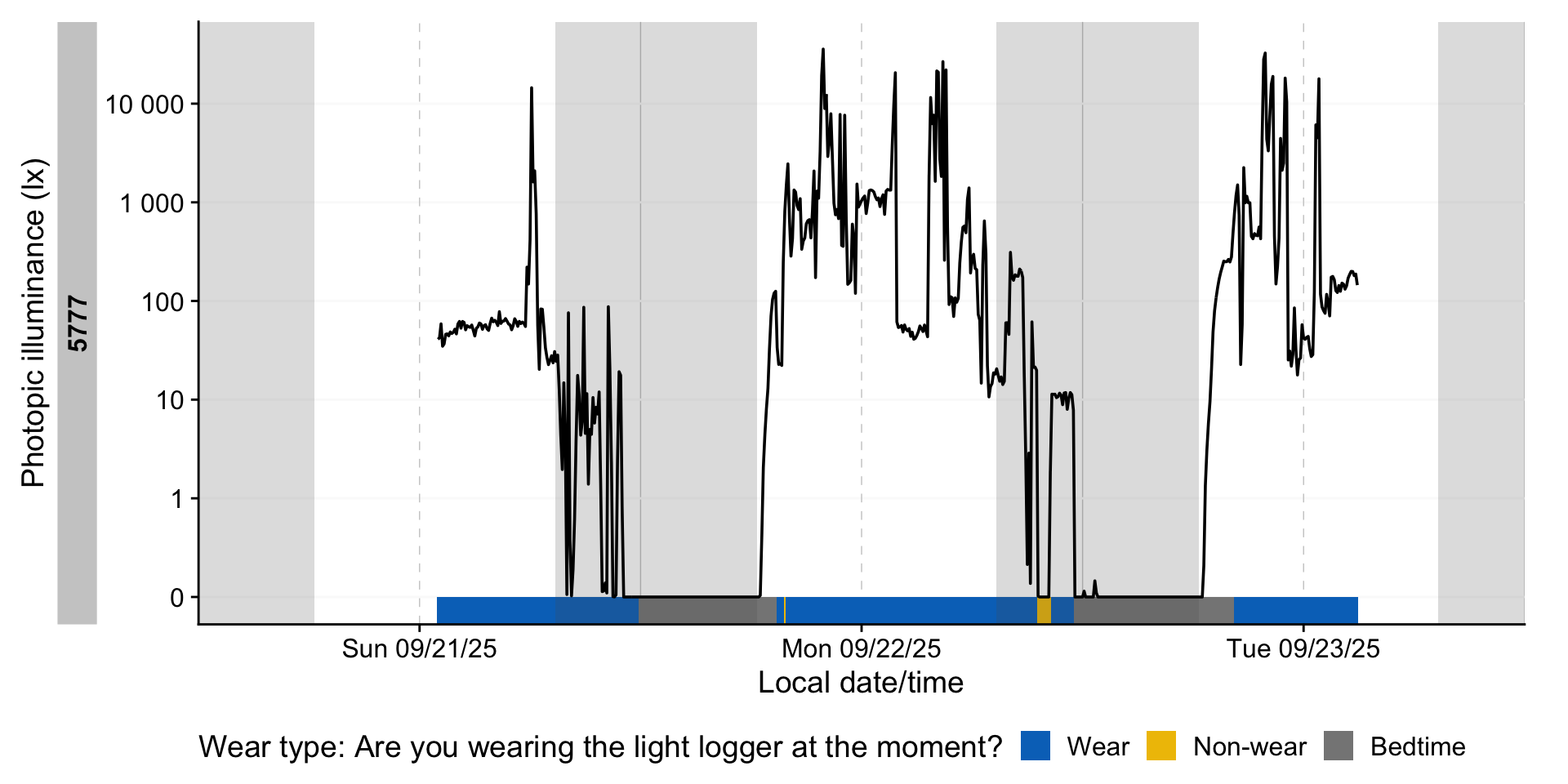
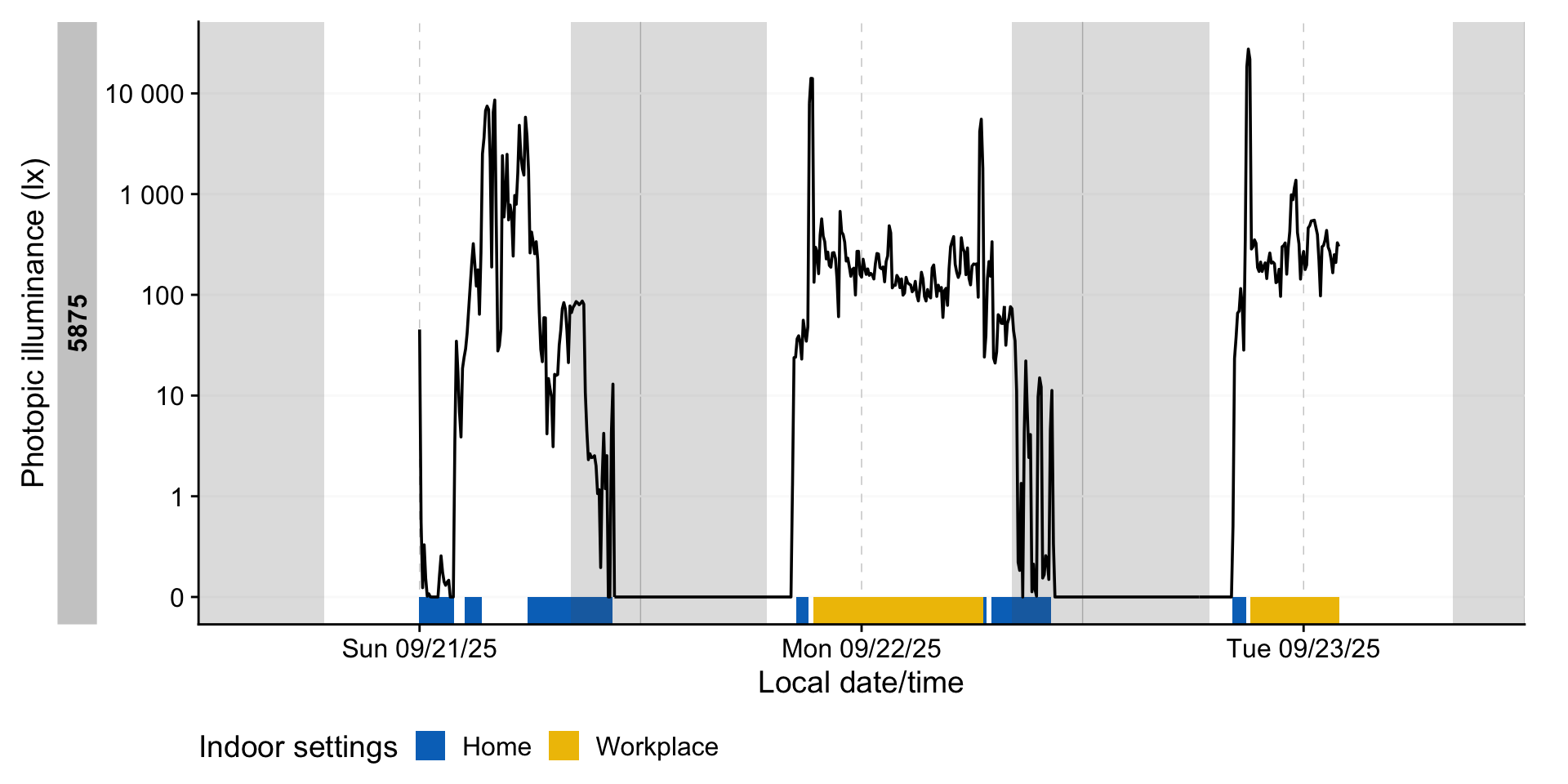
Next, we can visualize the activity logs together with the light information. To facilitate this, we again create a helper function. This opens a whole range of options to explore participants and states

state_plot <- function(variable, sample) {
light_data |>
    sample_groups(sample = sample) |> 
  gg_days(LIGHT, 
          x.axis = local_time,
          y.axis.label = "Photopic illuminance (lx)") |>
    gg_photoperiod(Datetime.colname = local_time) |> 
  gg_state({{ variable }}, aes_fill = {{ variable }}, 
           alpha = 1, ymax = 0, Datetime.colname = local_time) +
    theme_sub_legend(position = "bottom")
}
state_plot(setting_light, 6:7)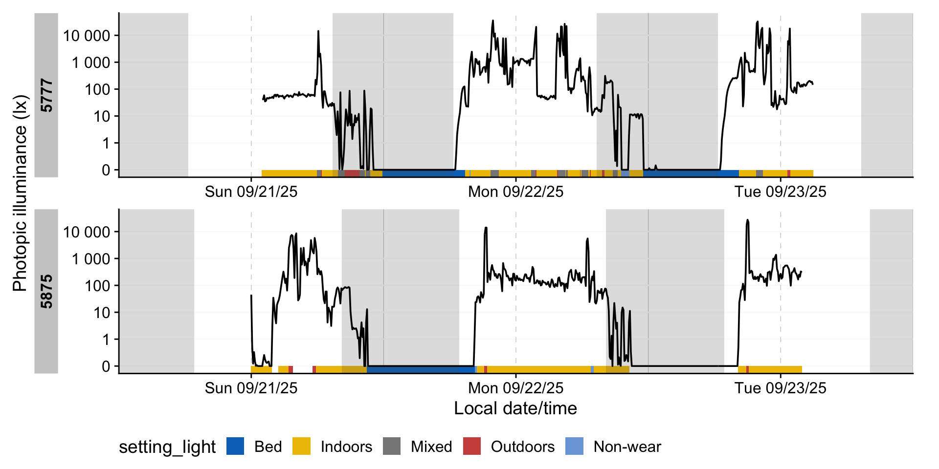

state_plot(type, 6)

state_plot(setting_indoors, 7)

7.2 Remove non-wear

As we now have logs of non-wear (both during the day and in sleep), we can set those measurements to NA.

light_data <-
  light_data |> 
  mutate(LIGHT = case_match(as.character(type),
                            c("Non-wear", "Bedtime") ~ NA_real_,
                            .default = LIGHT))

We can check whether we were successful, by summarizing our data depending on type.

light_data |> 
  group_by(type) |>
  summarize(mean = mean(LIGHT, na.rm = TRUE))

# A tibble: 4 × 2
  type      mean
  <fct>    <dbl>
1 Wear     1208.
2 Non-wear  NaN 
3 Bedtime   NaN 
4 <NA>      303.

This shows us that removing those instances was successful. To close up this use case, we can calculate a few metrics depending on the context with a helper function:

quick_summaries <- function(variable) {
light_data |> 
  group_by({{ variable }}, .add = TRUE) |>
1    durations(LIGHT, show.missing = TRUE, FALSE.as.NA = TRUE) |>
    ungroup(Id) |>
2    summarize_numeric(prefix = "mean_per_participant_") |>
3    extract_metric(
      light_data |>
        mutate({{ variable }} := factor({{ variable}})) |>
        group_by({{ variable }}
                 ),
4      identifying.colname = {{ variable }},
      Datetime.colname = local_time,
5      geo_mean = log_zero_inflated(LIGHT) |>
             mean(na.rm = TRUE) |>
             exp_zero_inflated()
      ) |>
    rename(participants = episodes) |> 
    drop_na() |>
    gt() |>
    fmt_number(geo_mean)
}

1: Calculate the duration of every state for each participant
2: Calculate the average duration per state across participants
3: We add the geometric mean to the summary with extract_metric, and supply the original dataset, grouped in the same way as our summary is
4: Secondary settings
5: The formula for the geometric mean uses log_zero_inflated() and its counterpart exp_zero_inflated() to allow for zero-lx values in the dataset

With this helper we can get quick overviews for many aspects:

quick_summaries(setting_light)

setting_light	mean_per_participant_duration	mean_per_participant_missing	mean_per_participant_total	total_duration	participants	geo_mean
Indoors	76660s (~21.29 hours)	5681s (~1.58 hours)	82340s (~22.87 hours)	3603000s (~5.96 weeks)	47	45.36
Mixed	15703s (~4.36 hours)	853s (~14.22 minutes)	16555s (~4.6 hours)	596700s (~6.91 days)	38	239.03
Outdoors	12364s (~3.43 hours)	255s (~4.25 minutes)	12619s (~3.51 hours)	581100s (~6.73 days)	47	559.38

quick_summaries(setting_indoors)

setting_indoors	mean_per_participant_duration	mean_per_participant_missing	mean_per_participant_total	total_duration	participants	geo_mean
Home	51098s (~14.19 hours)	6965s (~1.93 hours)	58063s (~16.13 hours)	2350500s (~3.89 weeks)	46	20.80
Workplace	30450s (~8.46 hours)	0s	30450s (~8.46 hours)	913500s (~1.51 weeks)	30	295.28
Education	5057s (~1.4 hours)	0s	5057s (~1.4 hours)	35400s (~9.83 hours)	7	416.78
Commercial	7488s (~2.08 hours)	324s (~5.4 minutes)	7812s (~2.17 hours)	187200s (~2.17 days)	25	116.97
Healthcare	3900s (~1.08 hours)	0s	3900s (~1.08 hours)	7800s (~2.17 hours)	3	468.57
Leisure	5130s (~1.43 hours)	270s (~4.5 minutes)	5400s (~1.5 hours)	51300s (~14.25 hours)	11	58.89
Other	4700s (~1.31 hours)	975s (~16.25 minutes)	5675s (~1.58 hours)	56400s (~15.67 hours)	13	57.92

quick_summaries(setting_outdoors)

setting_outdoors	mean_per_participant_duration	mean_per_participant_missing	mean_per_participant_total	total_duration	participants	geo_mean
Home	14876s (~4.13 hours)	18s	14894s (~4.14 hours)	252900s (~2.93 days)	18	227.70
Workplace	5127s (~1.42 hours)	82s (~1.37 minutes)	5209s (~1.45 hours)	56400s (~15.67 hours)	11	335.06
Education	750s (~12.5 minutes)	0s	750s (~12.5 minutes)	1500s (~25 minutes)	2	6,663.65
Commercial	3471s (~57.85 minutes)	0s	3471s (~57.85 minutes)	24300s (~6.75 hours)	8	576.79
Leisure	7436s (~2.07 hours)	332s (~5.53 minutes)	7768s (~2.16 hours)	208200s (~2.41 days)	28	745.51
Other	6062s (~1.68 hours)	44s	6106s (~1.7 hours)	206100s (~2.39 days)	36	680.07

quick_summaries(setting_mixed)

setting_mixed	mean_per_participant_duration	mean_per_participant_missing	mean_per_participant_total	total_duration	participants	geo_mean
Covered patio or terrace	10671s (~2.96 hours)	0s	10671s (~2.96 hours)	74700s (~20.75 hours)	9	59.17
Semi-open corridor/gallery	3900s (~1.08 hours)	660s (~11 minutes)	4560s (~1.27 hours)	19500s (~5.42 hours)	8	172.54
Balcony	1500s (~25 minutes)	0s	1500s (~25 minutes)	3000s (~50 minutes)	2	4.30
Veranda	24450s (~6.79 hours)	0s	24450s (~6.79 hours)	48900s (~13.58 hours)	3	339.81
Atrium	900s (~15 minutes)	0s	900s (~15 minutes)	900s (~15 minutes)	1	1,099.04
Transportation (car/taxi)	9970s (~2.77 hours)	290s (~4.83 minutes)	10260s (~2.85 hours)	299100s (~3.46 days)	30	583.61
Transportation (bus or commuter/regional rail)	3545s (~59.08 minutes)	300s (~5 minutes)	3845s (~1.07 hours)	39000s (~10.83 hours)	11	224.10
Transportation (long-distance train)	7800s (~2.17 hours)	0s	7800s (~2.17 hours)	31200s (~8.67 hours)	4	387.55
Transportation (underground, subway)	1350s (~22.5 minutes)	0s	1350s (~22.5 minutes)	5400s (~1.5 hours)	5	190.73
Transportation (airplane)	9750s (~2.71 hours)	150s (~2.5 minutes)	9900s (~2.75 hours)	39000s (~10.83 hours)	4	142.49
Transportation (bike)	14700s (~4.08 hours)	600s (~10 minutes)	15300s (~4.25 hours)	44100s (~12.25 hours)	3	29.25
Other	41933s (~11.65 hours)	200s (~3.33 minutes)	42133s (~11.7 hours)	377400s (~4.37 days)	10	212.83

quick_summaries(wear_activity)

wear_activity	mean_per_participant_duration	mean_per_participant_missing	mean_per_participant_total	total_duration	participants	geo_mean
Sedentary	64991s (~18.05 hours)	5221s (~1.45 hours)	70213s (~19.5 hours)	3054600s (~5.05 weeks)	47	52.97
Light activity	30430s (~8.45 hours)	1180s (~19.67 minutes)	31611s (~8.78 hours)	1399800s (~2.31 weeks)	46	136.54
Moderate activity	8150s (~2.26 hours)	350s (~5.83 minutes)	8500s (~2.36 hours)	244500s (~2.83 days)	30	162.56
High-intensity activity	6630s (~1.84 hours)	30s	6660s (~1.85 hours)	66300s (~18.42 hours)	10	130.65

8 Circular time

We close this use case off with with a small detour to averaging of times. Many calculations in wearable data analysis involves averaging. This is tricky for variables that are circular in nature, like the time of day. consider the following case:

times <- as.POSIXct(c("2025-12-07 23:59:00", "2025-12-09 00:01:00"))
times2 <- as.POSIXct(c("2025-12-06 23:59:00", "2025-12-09 00:01:00"))

When we take the average of these two, we get noon on 8 December.

mean(times)

[1] "2025-12-08 12:00:00 CET"

mean(times2)

[1] "2025-12-08 CET"

Depending on what the values represent, this is a correct handling. But consider they represent sleep times. In this case the averaging results to not output what we want, especially the sensitivity to the date for the result. We can lose the reliance on the date if we use a function like Datetime2Time() or summarize_numeric()s defaults:

tibble(times, times2) |> Datetime2Time()

# A tibble: 2 × 2
  times  times2
  <time> <time>
1 23:59  23:59 
2 00:01  00:01

tibble(times, times2) |> summarize_numeric()

# A tibble: 1 × 3
  mean_times mean_times2 episodes
  <time>     <time>         <int>
1 12:00      12:00              2

Now we have consistent results - but they are still wrong in the context we are thinking in. We need circular time for this, i.e., where the distance of two timepoints is equal, even across midnight. LightLogR has implemented functions from the circular package to make this process easy. Simply specify a circular handling. After the summary, apply Circular2Time() to backtransform to the common representation.

tibble(times, times2) |> Datetime2Time(circular = TRUE)

# A tibble: 2 × 2
  times       times2     
  <circular>  <circular> 
1 6.278821984 6.278821984
2 0.004363323 0.004363323

tibble(times, times2) |> 
  summarize_numeric(Datetime2Time.circular = TRUE) |> 
  Circular2Time()

# A tibble: 1 × 3
  mean_times    mean_times2   episodes
  <time>        <time>           <int>
1 00'00.000000" 00'00.000000"        2

We can use this approach in our use case. Say we want to know the average Bedtime of people, based on their logs:

bedtimes <- 
  events |> filter(type == "Bedtime") |> select(start) 
bedtimes |> head() |> gt()

start
2025-09-21 20:54:37
2025-09-22 19:46:08
2025-09-21 14:06:12
2025-09-22 00:28:40
2025-09-22 23:12:22
2025-09-22 19:36:30

Now focus on the difference of whether we work with circular time or not:

bedtimes |> summarize_numeric()

  mean_start episodes
1   16:42:13       88

bedtimes |> summarize_numeric(Datetime2Time.circular = TRUE) |> Circular2Time()

       mean_start episodes
1 23:03:48.132303       88

9 Conclusion

Congratulations! You have finished this section of the advanced course. If you go back to the homepage, you can select one of the other use cases.