Use case #02: Case, light sensitivity

Open and reproducible analysis of light exposure and visual experience data (Advanced)

Author

Affiliation

Johannes Zauner

Technical University of Munich & Max Planck Institute for Biological Cybernetics, Germany

Last modified:

December 8, 2025

1 Preface

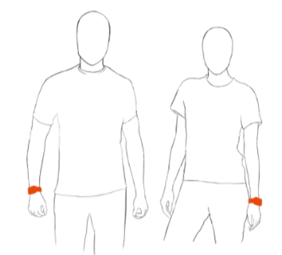
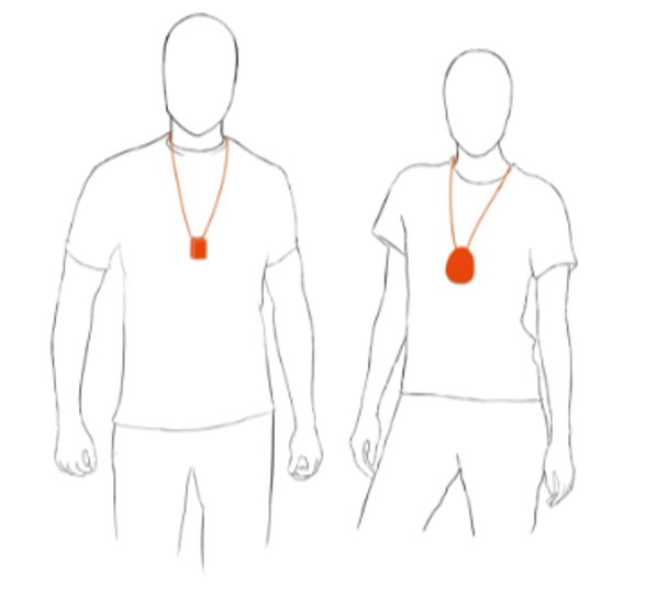
A single patient reports worse sleep after bright days. Consequently, personal light exposure and activity was captured with wearable devices for several weeks. Additionally, morning and evening questionnaires were used to capture sleep, performance, and well-being self evaluations. In this tutorial, we focus on the ActLumus device worn on the chest and the self evaluations.

The tutorial focuses on

import and merging of diary data with light data
calculation of metrics based on sleep-wake cycles instead of calendar days
relating exposure metrics to self assessments of consecutive sleep, performance, and wellbeing
assessing compliance to Brown et al. (2022)¹ recommendations

2 How this page works

This document contains the script for the online course series as a Quarto script, which can be executed on a local installation of R. Please ensure that all libraries are installed prior to running the script.

If you want to test LightLogR without installing R or the package, try the script version running webR, for a autonymous but slightly reduced version. These versions are indicated as (live), whereas the current version is considered (static), as it is pre-rendered.

To run this script, we recommend cloning or downloading the GitHub repository (link to Zip-file) and running the respective script. You will need to install the required packages. A quick way is to run:

renv::restore()

If this is your first course tutorial

This tutorial is considered as advanced. Basic functions in the LightLogR package as well as general tidy workflows are used without dedicated explanation. We recommend working through the beginner example if you are new to LightLogR (note that there is also a live variant).

3 Setup

We start by loading the necessary packages.

library(LightLogR) # main package
library(tidyverse) # for tidy data science
library(gt) # for great tables
library(readxl) # to read in Excel files
library(gtsummary) # for automatic summaries

4 Import

We require both light and log data to be loaded into R before we are able to merge them.

4.1 Light

Light data were captured with ActLumus devices. The exported data files sit in data/case_light_sensitivity/.

file <- "data/case_light_sensitivity/Log_5153_20251028143545799.txt"
tz <- "Europe/Berlin"
coordinates <- c(48.775555555556, 9.1827777777778247) #Stuttgart
1data <- import$ActLumus(file, tz = tz, manual.id = "ID001")

1: As there is only one participant, we set a manual Id


Successfully read in 34'735 observations across 1 Ids from 1 ActLumus-file(s).
Timezone set is Europe/Berlin.

First Observation: 2025-09-19 15:57:16
Last Observation: 2025-10-13 18:53:31
Data from before 2001-01-01 were not imported. Adjust with `not.before` if needed. 
Timespan: 24 days

Observation intervals: 
  Id    interval.time            n pct  
1 ID001 60s (~1 minutes)     34733 100% 
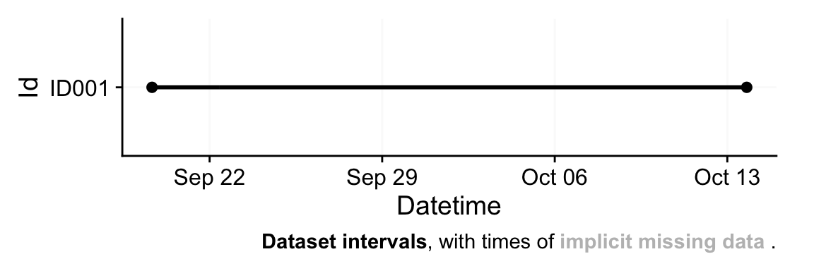
2 ID001 195s (~3.25 minutes)     1 0%

This dataset spans about three weeks. We know that the diaries only start on 24 September 2025 - thus we remove prior data. We also test for irregular data or gaps in this trimmed dataset.

data <- 
  data |> 
1  filter_Date(start = "2025-09-24") |>
2  ungroup() |>
  select(Datetime, MEDI) 
data |> has_gaps()
data |> has_irregulars()

1: If we have a hard-set beginning or end time, filter_Date() or filter_Datetime() provide convenient cut-off functionality.
2: As we are dealing with a single participant, we don’t require grouping by Id.

[1] FALSE
[1] FALSE

We can continue seeing as there are no issues with the regular time series. We start by plotting the full series

 data|> 
1  aggregate_Datetime("15 minutes") |>
2  gg_days(x.axis.format = "%a %d/%m") |>
  gg_photoperiod(coordinates)

1: Reduce the interval by averaging over 15 minute periods
2: Easily change the label format. Look at the help page of ?strptime for the available syntax.

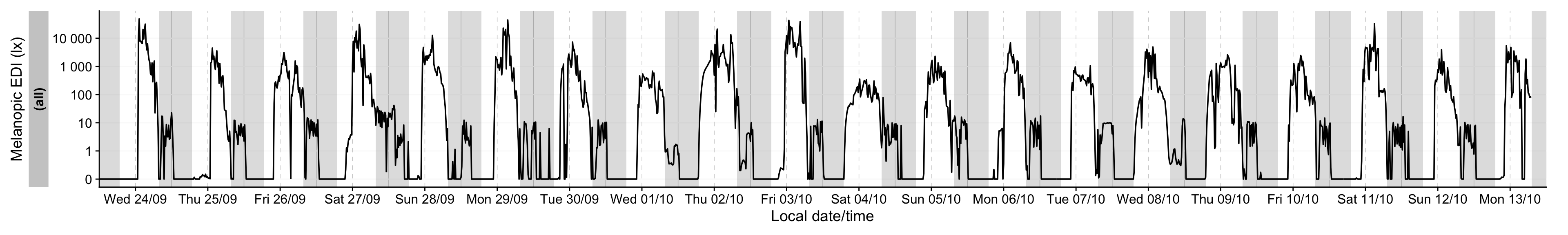
We can see the light intensity varies greatly. Let’s look at the extremes.

 data|> 
  aggregate_Datetime("5 minutes") |>
1  add_Date_col(group.by = TRUE) |>
2  sample_groups(n=3,
                order.by = 
                  duration_above_threshold(MEDI, Datetime, threshold = 250)
                  ) |>
  ungroup(Date) |> 
  gg_doubleplot(type = "repeat") |>
  gg_photoperiod(coordinates) +
  labs(title = "Three days with highest time above 250 lx mel EDI")

1: Adding, and grouping by, the date gives us 20 groups, each covering one calender day
2: Select the three groups with the highest duration above 250 lx mel EDI

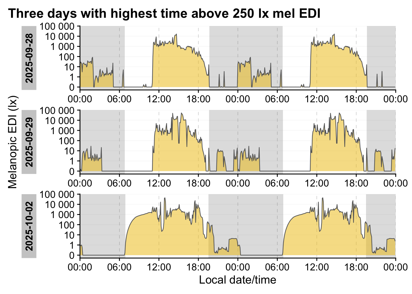
Looking at the first half of 02 October 2025, we can already see that this likely a period of non-wear, or sleep - this, we have to come back to later.

 data|> 
  aggregate_Datetime("5 minutes") |>
  add_Date_col(group.by = TRUE) |>
  sample_groups(n=3, 
1                sample = "bottom",
                order.by = 
                  duration_above_threshold(MEDI, Datetime, threshold = 250)
                ) |> 
  ungroup(Date) |> 
  gg_doubleplot(type = "repeat") |>
  gg_photoperiod(coordinates) +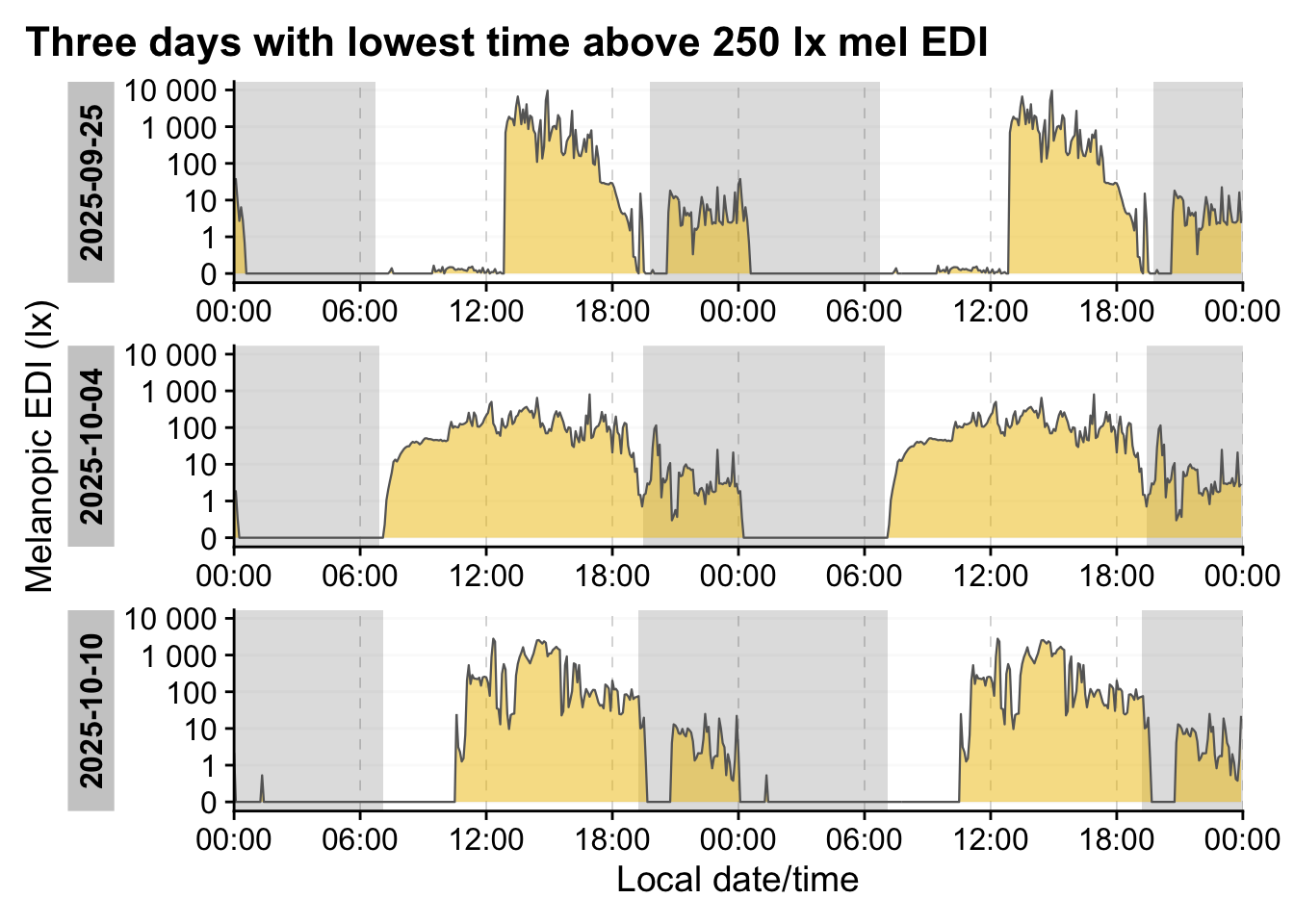
  labs(title = "Three days with lowest time above 250 lx mel EDI")

1: Select the three groups with the lowest duration above 250 lx mel EDI

4.2 State data

We need information about sleep times. These can be found in the diaries.

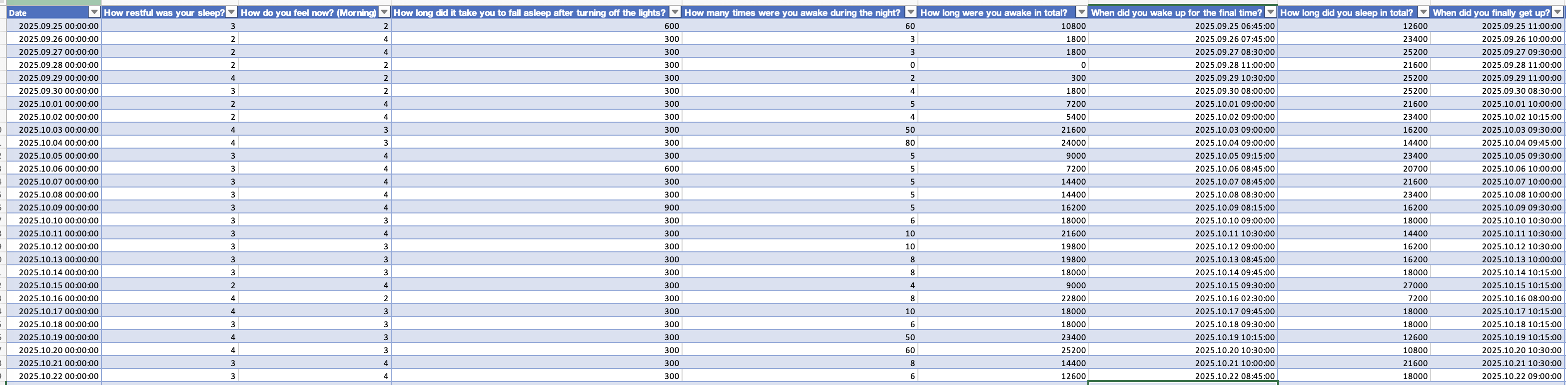
The morning diary is all about last nights sleep, how long the needed to fall asleep, wake-ups during the night, when they got up, how rested they feel and about sleep medication. See Figure 2 for an excerpt.

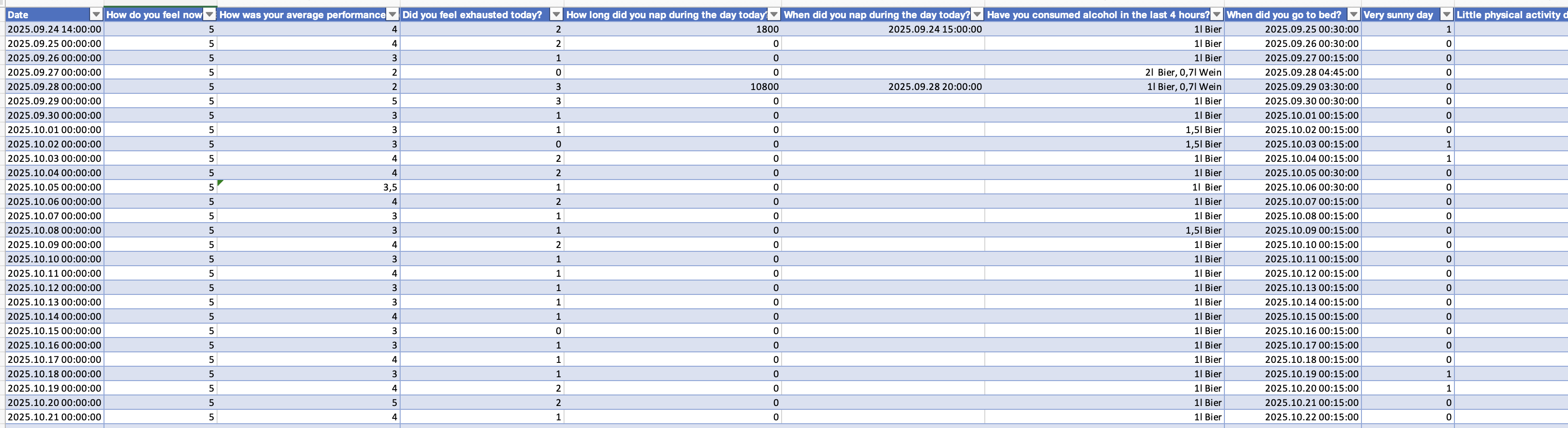
Figure 2: Excerpt from the morning diary as opened in Excel

Figure 3: Excerpt from the evening diary as opened in Excel

The evening diary is about the prior day, how well and they feel and about their performance during the day, alcohol consumation, when they got to bed, daytime naps and self-assessments about low activity and bright days. See Figure 3 for an excerpt.

In the next step we import these data and combine them to a large table. While none of these steps contain LightLogR functions, it is a crucial step to set the data up right for merging - particularly in that we assign the morning diaries to the prior day, and also add information about performance and fatigue on a given day to the prior day.

state_path1 <- "data/case_light_sensitivity/evening_protocol.xlsx"
state_path2 <- "data/case_light_sensitivity/morning_protocol.xlsx"

state_evening <- read_excel(state_path1)
state_morning <- read_excel(state_path2)

1state_evening$Date <- date(state_evening$Date)
state_morning$Date <- date(state_morning$Date - days(1))
2states <- left_join(state_evening, state_morning, by = "Date")

labels_states <- 
  names(states) |> 
  set_names(c("Date", "wellbeing.evening", "performance", "fatigue", 
              "daysleep.duration", "daysleep.start", "alcohol", "bedtime", 
              "sunny.day", "low.movement",
              "sleepquality", "wellbeing.morning", "sleepdelay", 
              "sleepinterruptions", "sleepinterruptions.duration", "wakeup", 
              "sleepduration", "outofbed", "medication"))
names(states) <- names(labels_states)

states <- 
3  states |> mutate(performance.next = lead(performance),
                   fatigue.next = lead(fatigue))

1: Store the date information of the evening diaries as is, but the morning diary will be set one day back.
2: By joining these two diaries by their (adjusted) date, morning diary information is related to the prior day evening diary.
3: We add the next days performance and fatigue level to all days.

The following table gives a short overview of the states. We will later get to whether a higher rating is better or worse for the individual items.

states |> 
  set_names(c(labels_states, "Performance next day", "Fatigue next day")) |>  
  tbl_summary(include = where(is.numeric))

Characteristic	N = 28¹
How do you feel now? (Evening)
5	28 (100%)
How was your average performance today?
2	2 (7.1%)
3	12 (43%)
3.5	1 (3.6%)
4	11 (39%)
5	2 (7.1%)
Did you feel exhausted today?
0	3 (11%)
1	15 (54%)
2	8 (29%)
3	2 (7.1%)
How long did you nap during the day today?
0	26 (93%)
1800	1 (3.6%)
10800	1 (3.6%)
Very sunny day	5 (18%)
Little physical activity during the day	5 (19%)
Unknown	1
How restful was your sleep?
2	6 (21%)
3	15 (54%)
4	7 (25%)
How do you feel now? (Morning)
2	5 (18%)
3	10 (36%)
4	13 (46%)
How long did it take you to fall asleep after turning off the lights?
300	25 (89%)
600	2 (7.1%)
900	1 (3.6%)
How many times were you awake during the night?	6 (5, 10)
How long were you awake in total?	14,400 (7,200, 19,800)
How long did you sleep in total?	18,000 (16,200, 23,400)
Have you taken any sleep medication since yesterday evening?
0	28 (100%)
Performance next day
2	2 (7.4%)
3	12 (44%)
3.5	1 (3.7%)
4	10 (37%)
5	2 (7.4%)
Unknown	1
Fatigue next day
0	3 (11%)
1	15 (56%)
2	7 (26%)
3	2 (7.4%)
Unknown	1
¹ n (%); Median (Q1, Q3)

5 Merging sleep data

Now that the diaries are prepared, we can extract sleep data from the states. The goal for the next code cell is to end with a statechange variable, that has a datetime for every timepoint when a new state occurs.

sleep_data <-
  states |>
1  mutate(sleep = bedtime + sleepdelay) |>
2  select(sleep, wake = wakeup) |>
3  pivot_longer(everything(), names_to = "state") |>
4  add_row(state = "wake",
          value = as.POSIXct("2025-09-24 14:00:00", tz = "UTC"),
          .before = 1)

1: Calculate sleep timing by adding bedtime and sleepdelay
2: Reduce the dataset to only sleep and wake times
3: We transform the data from wide to long format (i.e., consecutive wake-sleep statesd)
4: We add an initial wake for the first day

While we are at it, we can also create states according to the Brown et al. (2022) recommendations, which distinguish daytime (wake), evening (pre-sleep), and nighttime (sleep) hours. The LightLogR function sleep_int2Brown() makes this conversion a breeze. By default, the evening phase is set to a length of 3 hours.

sleep_data <-
  sleep_data |> 
1  sc2interval(value, state) |>
2  sleep_int2Brown(Brown.night = "sleep",
                  Brown.day = "wake",
                  Brown.evening = "pre-sleep")

1: Convert the statechanges into intervals, i.e. from datetimes when a state changes to intervals where a state is considered active.
2: Add a variable (State.Brown by default) containing the Brown et al. (2022) phases. This function automatically extends the rows to include the pre-sleep phase.

Next, we combine the light dataset with the sleep data.

data_ext <- 
data |> 
1  add_states(sleep_data,
2             start.colname = Interval,
             end.colname = Interval,
3             force.tz = TRUE) |>
4  drop_na(state) |>
  add_photoperiod(coordinates) |> 
  Brown2reference(
                  Brown.day = "wake",
                  Brown.evening = "pre-sleep",
                  Brown.night = "sleep")

data_ext |> head()

1: Combine the two datasets
2: Get the start and end datetimes for each state from the Interval column
3: Assures that the times from the sleep_data dataset are matched up with the light data, even though the light data uses the Central European Time, whereas the sleep states use the default UTC time zone.
4: Remove times that don’t relate to any state

# A tibble: 6 × 12
  Datetime             MEDI state State.Brown dawn               
  <dttm>              <dbl> <chr> <chr>       <dttm>             
1 2025-09-24 14:00:31 6896. wake  wake        2025-09-24 06:41:25
2 2025-09-24 14:01:31 6895. wake  wake        2025-09-24 06:41:25
3 2025-09-24 14:02:31 6867. wake  wake        2025-09-24 06:41:25
4 2025-09-24 14:03:31 6845. wake  wake        2025-09-24 06:41:25
5 2025-09-24 14:04:31 6790. wake  wake        2025-09-24 06:41:25
6 2025-09-24 14:05:31 6749. wake  wake        2025-09-24 06:41:25
# ℹ 7 more variables: dusk <dttm>, photoperiod <drtn>, photoperiod.state <chr>,
#   Reference <dbl>, Reference.check <lgl>, Reference.difference <dbl>,
#   Reference.label <chr>

6 Brown et al. (2022) recommendations

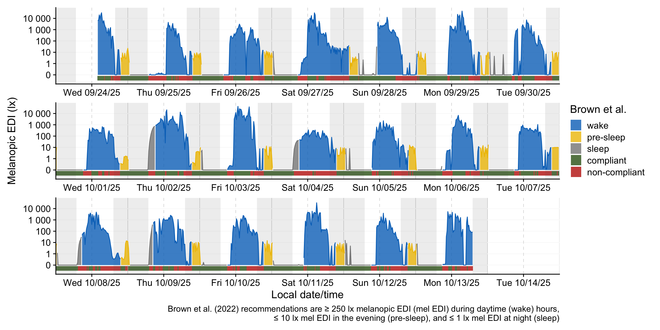
Let’s visualize the newly extended dataset with regards to the Brown et al. (2022) states.

color_palette <-
  c(
    wake =           "#0073C2FF",
    `pre-sleep` =    "#EFC000FF",
    sleep =          "#868686FF",
    compliant =      "#658354",
    `non-compliant` = "#CD534CFF"
  )

data_ext |>
  aggregate_Datetime("15 mins") |>
1  mutate(week = week(Datetime),
         week = paste0("week: ", week),
         Reference.check = 
           case_when(Reference.check ~ "compliant",
                     !Reference.check ~ "non-compliant"),
2         State.Brown = fct_expand(State.Brown, "compliant", "non-compliant") |>
                       fct_relevel("wake")
  ) |> 
  group_by(week) |>
3  gg_days(geom = "ribbon",
          alpha = 0.8,
          lwd = 0.5,
4          aes_col = State.Brown,
          aes_fill = State.Brown,
          group = consecutive_id(State.Brown),
5          x.axis.limits = \(x) {
            Datetime_limits(x, length = ddays(6), midnight.rollover = TRUE)
            }
          ) |> 
  gg_photoperiod(alpha = 0.1) |> 
6  gg_states(Reference.check,
            aes_fill = Reference.check,
7            ymax = -0.1, ymin = -0.5,
            alpha = 1) + 
  labs(fill = "Brown et al.",
       caption = 
         "Brown et al. (2022) recommendations are ≥ 250 lx melanopic EDI (mel EDI) during daytime (wake) hours,\n≤ 10 lx mel EDI in the evening (pre-sleep), and ≤ 1 lx mel EDI at night (sleep)") +
  guides(color = "none") +
  scale_fill_manual(values = color_palette) +
8  theme_sub_strip(background = element_blank(),
                  text.y = element_blank())

1: Grouping by week so that the plot is automatically sectioned into three rows
2: The expansion of factor levels is purely so that the order in the legend is automatically kept in sensible order.
3: Setting the geom to ribbon enables a filled band with the lower band set at 0.
4: Coloring and filling by the Brown states will only look good, if each section is kept individually. consecutive_id() ensures just this.
5: Manually setting the datetime limits ensures that each row is kept at 7 days
6: We add a check whether the recommendations were fulfilled and color by it.
7: Adjusting the height of the state bands ensures readability of the plot despite other color aspects.
8: As the week grouping is just for row-setting, we are not interested in the strip and thus remove it.

We can further summarize the compliance to the recommendations in a table.

data_ext |> 
  group_by(State.Brown) |> 
  summarize(`Relative compliance` = sum(Reference.check)/n(),
            `Relative duration` = n()) |> 
  mutate(`Relative duration` = `Relative duration` / sum(`Relative duration`),
         State.Brown = fct_relevel(State.Brown, "wake")
  ) |> 
  arrange(State.Brown) |> 
  gt() |> 
  fmt_percent(decimals = 0)

State.Brown	Relative compliance	Relative duration
wake	35%	54%
pre-sleep	89%	12%
sleep	95%	33%

7 Calculate metrics

In this section, we calculate some light metrics that we can correlate with sleep quality. We calculate these metrics not by the 24-hour day, but rather by wake-sleep rhythms.

7.1 Sleep-wake cycles

data_sw <-
data_ext |> 
  add_Date_col() |> 
1  number_states(state, use.original.state = FALSE) |>
  mutate(
2    sleep.wake = sprintf("cycle %02.f", state.count) |> factor(),
    .before = 1) |> 
  group_by(sleep.wake)

data_sw |> head()

1: Create a consecutive numbering per sleep-wake cycle. Beware if states are missing in other analyses!
2: Format the sleep-wake cycles nicely

# A tibble: 6 × 15
# Groups:   sleep.wake [1]
  sleep.wake Datetime             MEDI state State.Brown dawn               
  <fct>      <dttm>              <dbl> <chr> <chr>       <dttm>             
1 cycle 01   2025-09-24 14:00:31 6896. wake  wake        2025-09-24 06:41:25
2 cycle 01   2025-09-24 14:01:31 6895. wake  wake        2025-09-24 06:41:25
3 cycle 01   2025-09-24 14:02:31 6867. wake  wake        2025-09-24 06:41:25
4 cycle 01   2025-09-24 14:03:31 6845. wake  wake        2025-09-24 06:41:25
5 cycle 01   2025-09-24 14:04:31 6790. wake  wake        2025-09-24 06:41:25
6 cycle 01   2025-09-24 14:05:31 6749. wake  wake        2025-09-24 06:41:25
# ℹ 9 more variables: dusk <dttm>, photoperiod <drtn>, photoperiod.state <chr>,
#   Reference <dbl>, Reference.check <lgl>, Reference.difference <dbl>,
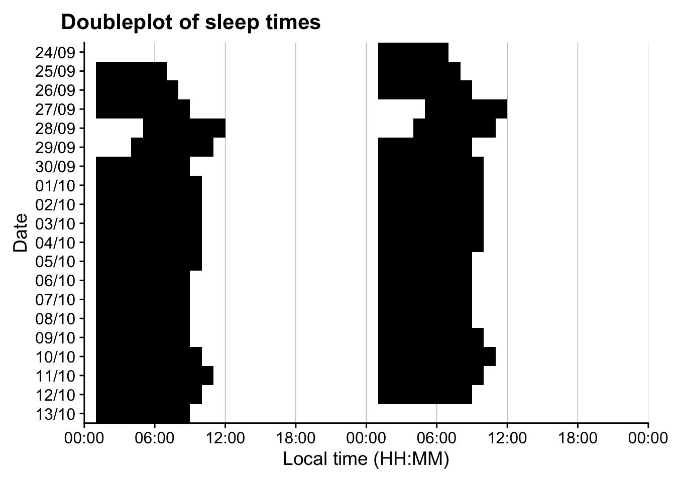
#   Reference.label <chr>, Date <date>, state.count <int>

Let’s look at the sleep times as a doubleplot.

data_sw |> 
  ungroup() |>
1  gg_heatmap(state == "sleep",
2             doubleplot = "next",
3             fill.remove = TRUE) +
  scale_fill_manual(values = c("TRUE" = "black", "FALSE" = "#00000000")) +
  guides(fill = "none") +
  labs(title = "        Doubleplot of sleep times") +
  theme(
  strip.background = element_blank(),
  strip.text.y = element_blank(),
  strip.placement = "inside")

1: Create a logical as the main variable that is TRUE when the state is sleep
2: Showing the next day in the doubleplot
3: Remove the default fill settings to provide your own

Again, we can look at the data as a table.

data_sw |> durations() |> ungroup() |> gt()

sleep.wake	duration
cycle 01	60300s (~16.75 hours)
cycle 02	90000s (~1.04 days)
cycle 03	89100s (~1.03 days)
cycle 04	95400s (~1.1 days)
cycle 05	84600s (~23.5 hours)
cycle 06	77400s (~21.5 hours)
cycle 07	90000s (~1.04 days)
cycle 08	86400s (~1 days)
cycle 09	86400s (~1 days)
cycle 10	86400s (~1 days)
cycle 11	87300s (~1.01 days)
cycle 12	84600s (~23.5 hours)
cycle 13	86400s (~1 days)
cycle 14	85500s (~23.75 hours)
cycle 15	85500s (~23.75 hours)
cycle 16	89100s (~1.03 days)
cycle 17	91800s (~1.06 days)
cycle 18	81000s (~22.5 hours)
cycle 19	85500s (~23.75 hours)
cycle 20	36480s (~10.13 hours)

Based on these results, we will remove cycle 01 and cycle 20, as they have only partial data.

data_sw <-
  data_sw |> filter(!sleep.wake %in% c("cycle 01", "cycle 20"))

7.2 Light exposure metrics

For the last step, we will calculate two relevant light exposure metrics, time above 250 lx mel EDI and dose. and add this information to the original states.

summaries_sw <- 
data_sw |> 
  summarize(
1    Date = min(Date),
    dose(MEDI, Datetime, as.df = TRUE),
    duration_above_threshold(MEDI, Datetime, threshold = 250, as.df = TRUE)
  ) |> 
2  left_join(states, by = "Date")

1: This step relates the sleep cycles to the date where the wake-state starts.
2: Adding the self-assessments to our summaries. The data (4) provides the right assignment.

We bring this information together into a comprehensive table. Variables that have no meaningful variance are removed.

summaries_sw |> 
  select(Date, sleep.wake, dose, duration_above_250,
         wellbeing.morning, sunny.day, low.movement, performance, 
         fatigue, bedtime, sleepquality, sleepduration, 
         sleepinterruptions, sleepinterruptions.duration) |> 
  gt() |> 
  fmt_number(dose, decimals = 0) |>
  fmt_duration(c(duration_above_250, sleepduration, sleepinterruptions.duration), 
               input_units = "seconds") |> 
  fmt_time(bedtime) |> 
  fmt(c(sunny.day, low.movement), fns = \(x) ifelse(x, "Yes", "No")) |> 
  tab_header("Overview of daily light exposure metrics and key questionnaire data") |> 
  tab_spanner("Light exposure", columns = c(dose, duration_above_250)) |> 
  tab_spanner("Self-report", columns = wellbeing.morning:fatigue) |> 
  tab_spanner("Self-reported sleep", columns = bedtime:sleepinterruptions.duration) |> 
  cols_label(sleep.wake = "Sleep-wake",
             dose = "Dose mel EDI (lx·h)",
             duration_above_250 = "Time above 250lx mel EDI",
             wellbeing.morning = "Wellbeing next morning",
             sunny.day = "Sunny day",
             low.movement = "Low activity",
             performance = "Performance",
             fatigue = "Fatigue",
             bedtime = "Bedtime",
             sleepquality = "Sleep quality",
             sleepduration = "Sleep duration",
             sleepinterruptions = "Sleep interruptions",
             sleepinterruptions.duration = "Interruption duration"
             ) |> 
  tab_footnote("Higher is worse", locations = cells_column_labels(c(8, 9, 11, 13, 14))) |> 
  sub_missing()

Date	Sleep-wake	Light exposure		Self-report					Self-reported sleep
Overview of daily light exposure metrics and key questionnaire data
Date	Sleep-wake	Dose mel EDI (lx·h)	Time above 250lx mel EDI	Wellbeing next morning	Sunny day	Low activity	Performance¹	Fatigue¹	Bedtime	Sleep quality¹	Sleep duration	Sleep interruptions¹	Interruption duration¹
2025-09-25	cycle 02	6,075	3h 8m	4	No	No	4.0	2	00:30:00	2	6h 30m	3	30m
2025-09-26	cycle 03	5,936	5h 16m	4	No	No	3.0	1	00:15:00	2	7h	3	30m
2025-09-27	cycle 04	32,863	5h 3m	2	No	No	2.0	0	04:45:00	2	6h	0	0s
2025-09-28	cycle 05	14,993	6h 28m	2	No	No	2.0	3	03:30:00	4	7h	2	5m
2025-09-29	cycle 06	42,373	5h 22m	2	No	Yes	5.0	3	00:30:00	3	7h	4	30m
2025-09-30	cycle 07	9,481	4h 46m	4	No	Yes	3.0	1	00:15:00	2	6h	5	2h
2025-10-01	cycle 08	2,832	4h 46m	4	No	No	3.0	1	00:15:00	2	6h 30m	4	1h 30m
2025-10-02	cycle 09	31,293	8h 3m	3	Yes	No	3.0	0	00:15:00	4	4h 30m	50	6h
2025-10-03	cycle 10	70,280	5h 29m	3	Yes	No	4.0	2	00:15:00	4	4h	80	6h 40m
2025-10-04	cycle 11	1,493	1h 33m	4	No	No	4.0	2	00:30:00	3	6h 30m	5	2h 30m
2025-10-05	cycle 12	4,222	4h 40m	4	No	—	3.5	1	00:30:00	3	5h 45m	5	2h
2025-10-06	cycle 13	9,246	4h 35m	4	No	Yes	4.0	2	00:15:00	3	6h	5	4h
2025-10-07	cycle 14	3,053	5h 13m	4	No	Yes	3.0	1	00:15:00	3	6h 30m	5	4h
2025-10-08	cycle 15	8,892	3h 25m	4	No	No	3.0	1	00:15:00	3	4h 30m	5	4h 30m
2025-10-09	cycle 16	6,585	4h 48m	3	No	No	4.0	2	00:15:00	3	5h	6	5h
2025-10-10	cycle 17	4,446	3h 18m	4	No	No	3.0	1	00:15:00	3	4h	10	6h
2025-10-11	cycle 18	24,397	4h 3m	3	No	No	4.0	1	00:15:00	3	4h 30m	10	5h 30m
2025-10-12	cycle 19	4,020	3h 14m	3	No	No	3.0	1	00:15:00	3	4h 30m	8	5h 30m
¹ Higher is worse

8 Correlations

To visualize simple correlations between the self-assessments and the light exposure metrics we create a helper function:

time2hour <- function(x) x/3600
correlation_plot <- function(variable, label) {
  summaries_sw |> 
  #prepare the light exposure variables and bedtime variable:
  mutate(
    bedtime = hms::as_hms(bedtime) |> as.numeric() |> time2hour(),
    duration_above_250 = as.numeric(duration_above_250),
    duration_above_250 = 
      (duration_above_250 - min(duration_above_250))/
      (max(duration_above_250)-min(duration_above_250))*max(dose)/1000,
    dose = dose/1000
         ) |> 
  #create the ggplot:
  ggplot(aes(y = {{ variable }})) +
  geom_smooth(method = "lm", 
              aes(x = dose), 
              col = "#2E6F40", 
              fill = "#2E6F40") +
  geom_smooth(method = "lm", 
              aes(x = duration_above_250), 
              col = "#990011", 
              fill = "#990011") +
  geom_point(aes(x = dose), 
             col = "#2E6F40") +
  geom_point(aes(x = duration_above_250), 
             col = "#990011", size = 1) +
  scale_x_continuous(
    "Melanopic EDI dose (klx·h)",
    sec.axis = sec_axis(~ (.*1000/70280*23400 - 5580)/3600, 
                        name = "Time above 250 lx (h)")
  ) +
  cowplot::theme_cowplot() +
  theme_sub_axis_bottom(title = element_text(color = "#2E6F40"),
                        text = element_text(color = "#2E6F40")) +
  theme_sub_axis_top(title = element_text(color = "#990011"),
                        text = element_text(color = "#990011")) +
  labs(y = label) 
}

This allows us to easily look at the various parameters

correlation_plot(wellbeing.morning, 
                 "Wellbeing on the next\nmorning (higher = better)")

correlation_plot(sleepquality, "Sleep quality\n(higher = worse")

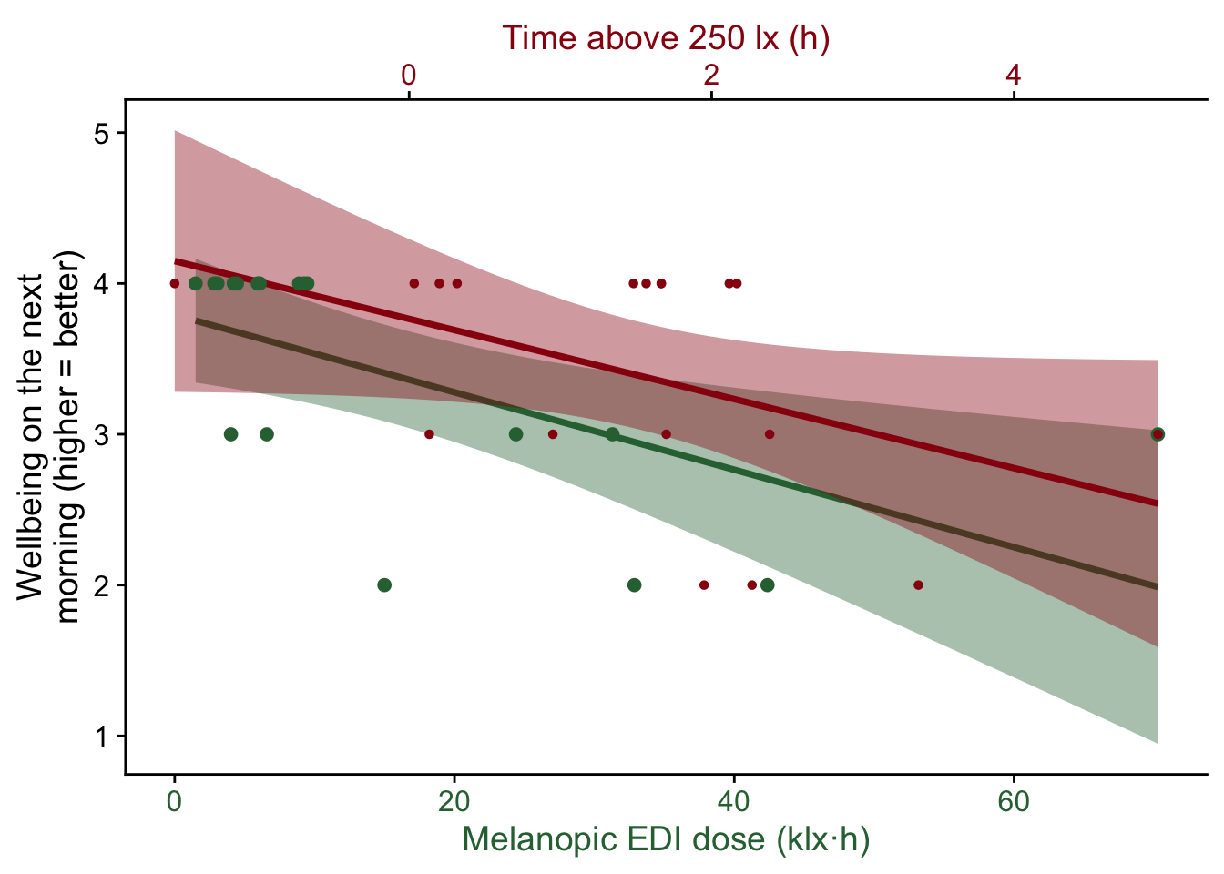
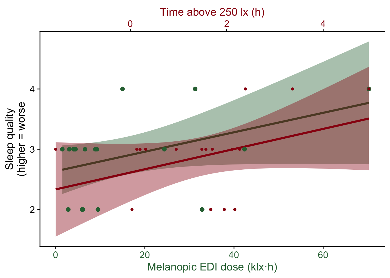
Try these for yourself. Could there be a meaningful relationship?

correlation_plot(performance, "Performance during\nthe day (higher = worse)")
correlation_plot(performance.next, 
                 "Performance on the\n next day (higher = worse)")
correlation_plot(sleepduration/3600, "Sleep duration (h)")
correlation_plot(fatigue, "Fatigue during the day\n(higher = worse)")
correlation_plot(fatigue.next, "Fatigue on the next day\n(higher = worse)")
correlation_plot(sleepinterruptions, "Sleep interruptions")
correlation_plot(sunny.day, "Self-assessed sunny day")
correlation_plot(low.movement, "Self-assessed low activity")

9 Conclusion

Congratulations! You have finished this section of the advanced course. If you go back to the homepage, you can select one of the other use cases.

Footnotes

Link to publication ↩︎