Use case #03: Light therapy

Open and reproducible analysis of light exposure and visual experience data (Advanced)

Author

Affiliation

Johannes Zauner

Technical University of Munich & Max Planck Institute for Biological Cybernetics, Germany

Last modified:

December 8, 2025

1 Preface

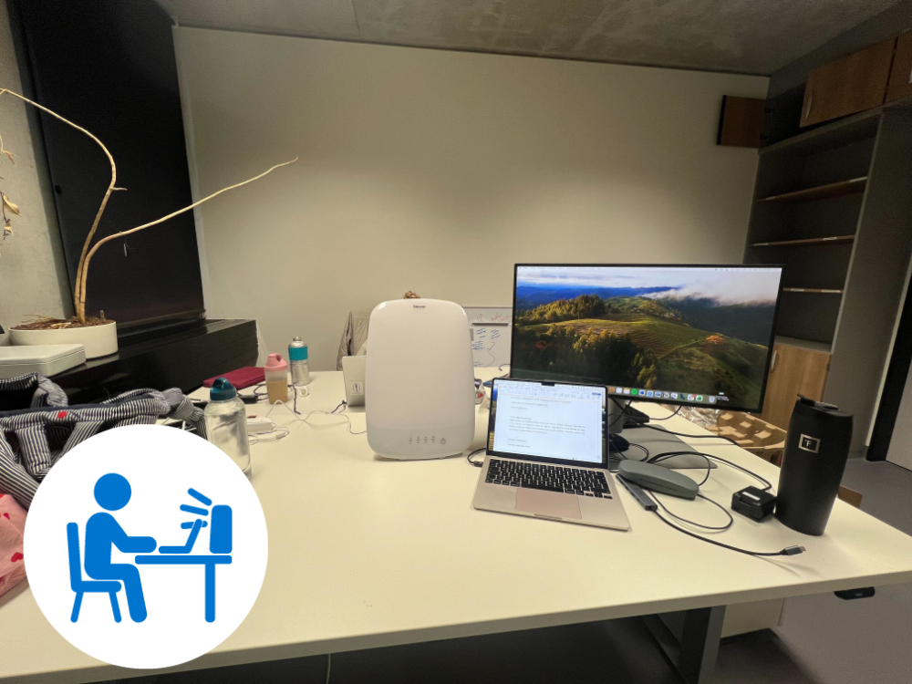
This use case covers an exploratory protocol to capture the effect of a light therapy intervention on personal light exposure. Two participants sit in an office environment, one with, one without a therapy lamp on their respective desk. They follow a typical office workflow. The blinds are shut to reduce the directional (and thus differential) effect of daylight on participant’s light exposure. Artificial lighting is switched on. In the intervention condition the therapy lamp is switched on for one hour. The participants document the start and end times of each protocol phase (pre-light, therapy light, post-light), as well as any deviations from the protocol.

Therapy light workplace (therapy light switched off)

The tutorial focuses on

merging of participant protocol logs with light from a wearable device
analysis of light exposure dependent on lighting conditions
dealing with interruptions from the protocol
advanced plotting & table styling
working with data < 1 day in LightLogR

2 How this page works

This document contains the script for the online course series as a Quarto script, which can be executed on a local installation of R. Please ensure that all libraries are installed prior to running the script.

If you want to test LightLogR without installing R or the package, try the script version running webR, for a autonymous but slightly reduced version. These versions are indicated as (live), whereas the current version is considered (static), as it is pre-rendered.

To run this script, we recommend cloning or downloading the GitHub repository (link to Zip-file) and running the respective script. You will need to install the required packages. A quick way is to run:

renv::restore()

If this is your first course tutorial

This tutorial is considered as advanced. Basic functions in the LightLogR package as well as general tidy workflows are used without dedicated explanation. We recommend working through the beginner example if you are new to LightLogR (note that there is also a live variant).

3 Setup

We start by loading the necessary packages.

library(LightLogR) # main package
library(tidyverse) # for tidy data science
library(gt) # for great tables
library(legendry) # for advanced legend manipulation
library(readxl) # to read in Excel files
library(ggridges) # for stacked plots within a panel
library(ggimage) # to add images to plots

4 Import

We require both light and log data to be loaded into R before we are able to merge them.

4.1 Light

Light data were captured with ActLumus devices. The exported data files sit in data/light_therapy/.

path <- "data/light_therapy"
files <- list.files(path, pattern = ".txt$", full.names = TRUE)
1pattern <- "Log_(.{4})_"
tz <- "Europe/Berlin"
data <- import$ActLumus(files, tz = tz, auto.id = pattern)

1: Pattern to extract Id’s from file names


Successfully read in 318 observations across 2 Ids from 2 ActLumus-file(s).
Timezone set is Europe/Berlin.

First Observation: 2025-10-30 09:46:36
Last Observation: 2025-10-30 12:26:50
Timespan: 2.7 hours

Observation intervals: 
  Id    interval.time        n pct  
1 4789  60s (~1 minutes)   160 100% 
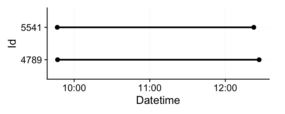
2 5541  60s (~1 minutes)   156 100%

We can see that it is a small dataset. If we visualize it we can see both participants measured simultaneously in the morning.

coordinates <- c(48.1371, 11.5754) #data were captured in Munich, Germany
data |> 
  gg_day(aes_col = fct_rev(Id)) |> 
  gg_photoperiod(coordinates)

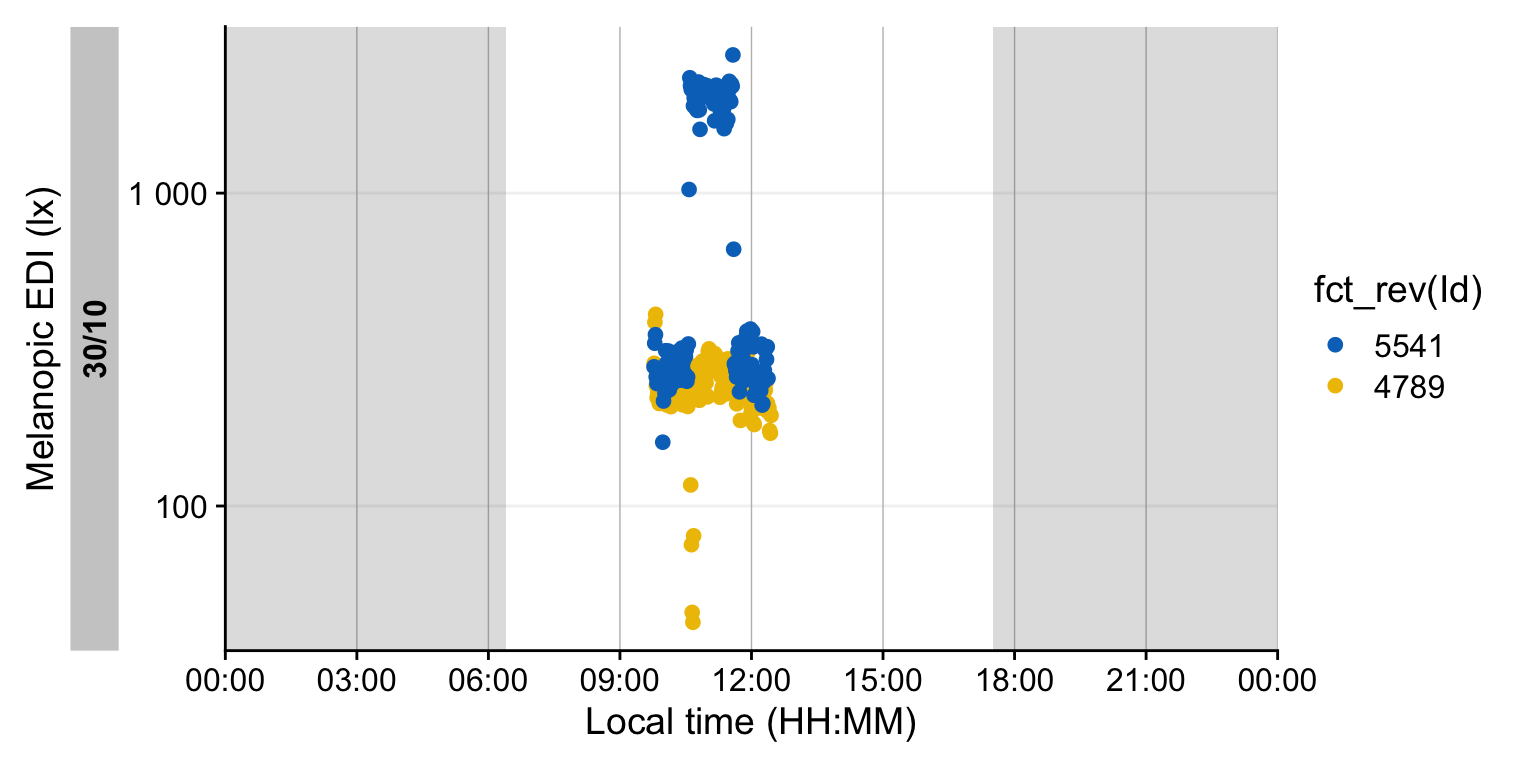
Participant 5541 received the therapy light, and 4789 is the control condition.

While the import summary did not show indications of gaps or irregular data, it always pays to check this.

data |> 
1  gap_table(full.days = FALSE) |>
2  cols_hide(contains("_n"))

1: As we have less than one day of data, it would not be sensible to check for missing data with regards to a full day.
2: Hides a few columns which are unnecessary here

	Data					Missing
Summary of available and missing data
Variable: melanopic EDI
	Regular		Irregular	Range	Interval	Gaps				Implicit		Explicit
	Time	%	n^1,2	Time	Time	N	ø	Time	%	Time	%	Time	%
Overall	5h 18m	100.0%³	0	5h 18m	60	0	0s	0s	0.0%³	0s	0.0%³	0s	0.0%³
4789
	2h 41m	100.0%	0	2h 41m	60s (~1 minutes)	0	0s	0s	0.0%	0s	0.0%	0s	0.0%
5541
	2h 37m	100.0%	0	2h 37m	60s (~1 minutes)	0	0s	0s	0.0%	0s	0.0%	0s	0.0%
¹ If n > 0: it is possible that the other summary statistics are affected, as they are calculated based on the most prominent interval.
² Number of (missing or actual) observations
³ Based on times, not necessarily number of observations

4.2 Logs

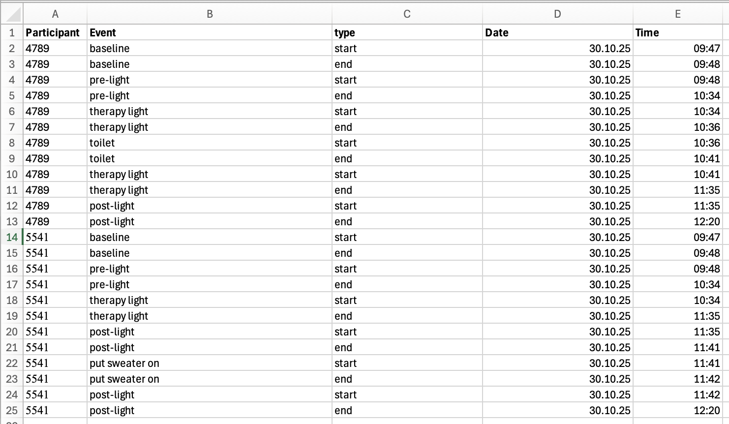
Participant logs are stored in a consolidated Excel file. Figure 2 shows the contents of the files when opened in Excel.

On pre-cleaning of manually entered content (logs/diaries)

Note that pre-cleaning was performed to ensure consistent naming and formatting. I have yet to come upon an experiment with manually entered content in the form of logs or diaries that required no cleaning whatsoever.

The utility of these data depend heavily on these factors, some of which can be changed after import:

Identical naming of grouping variables between wearable devices and logs. If there are even slight differences, like an additional whitespace ” “, the merge will be lossy.
Date, time, and datetime formats must be absolutely consistent and follow a standard formatting convention. If there are differences, they will be read in as text and parsing whole columns to the desired format can be lossy.

Figure 2: Participant log as opened in Excel

path <- "data/light_therapy/event_log_LightLamp.xlsx"
state_data <- read_excel(path)
state_data |> group_by(Participant) |>  slice_head(n=2)

# A tibble: 4 × 5
# Groups:   Participant [2]
  Participant Event    type  Date                Time               
        <dbl> <chr>    <chr> <dttm>              <dttm>             
1        4789 baseline start 2025-10-30 00:00:00 1899-12-31 09:47:00
2        4789 baseline end   2025-10-30 00:00:00 1899-12-31 09:48:00
3        5541 baseline start 2025-10-30 00:00:00 1899-12-31 09:47:00
4        5541 baseline end   2025-10-30 00:00:00 1899-12-31 09:48:00

Next we need to make adjustments to naming and types of variables. Note that the time variable is already recognized as a datetime, but with a nonsensical date.

state_data <-
  state_data |> 
1    rename(Id = Participant, state = Event) |>
2    mutate(Datetime = `date<-`(Time, Date),
           Id = factor(Id)) |>
    select(-Date, -Time) |>
3    number_states(type, use.original.state = FALSE) |>
4    pivot_wider(id_cols = c(Id, state, type.count), values_from = Datetime,
                names_from = type) |>
    select(-type.count) |> 
  group_by(Id)

1: Use naming conventions from LightLogR
2: Create a datetime that takes the Time variable (which is already recognized as a datetime) and just replace the Date component. Id is changed to a factor, and unnecessary columns are dropped
3: Number the type column by increasing the number with each start and end combo.
4: Pivot the dataset so that we end up with a start and end datetime for each state.

Let’s get an overview of our states before merging.

state_data |> 
  gt(rowname_col = "state") |> 
  tab_footnote(
    ("Note that only ID 5541 received the therapy light intervention, 
     but the time span it was active in the room is denoted in both 
     state datasets"), 
    locations = cells_stub(contains("therapy light"))
    )

	start	end
4789
baseline	2025-10-30 09:47:00	2025-10-30 09:48:00
pre-light	2025-10-30 09:48:00	2025-10-30 10:34:00
therapy light¹	2025-10-30 10:34:00	2025-10-30 10:36:00
toilet	2025-10-30 10:36:00	2025-10-30 10:41:00
therapy light¹	2025-10-30 10:41:00	2025-10-30 11:35:00
post-light	2025-10-30 11:35:00	2025-10-30 12:20:00
5541
baseline	2025-10-30 09:47:00	2025-10-30 09:48:00
pre-light	2025-10-30 09:48:00	2025-10-30 10:34:00
therapy light¹	2025-10-30 10:34:00	2025-10-30 11:35:00
post-light	2025-10-30 11:35:00	2025-10-30 11:41:00
put sweater on	2025-10-30 11:41:00	2025-10-30 11:42:00
post-light	2025-10-30 11:42:00	2025-10-30 12:20:00
¹ Note that only ID 5541 received the therapy light intervention, but the time span it was active in the room is denoted in both state datasets

5 Combine light and log data

Combining wearable data with state data is very easy, once both datasets have been properly prepared.

# states to keep
states_to_keep <- c("pre-light", "therapy light", "post-light", "baseline")
data <-
  data |> 
  select(Id, Datetime, MEDI) |> 
1  add_states(state_data, force.tz = TRUE) |>
  mutate(state = state |> 
2                  factor(levels = states_to_keep,
                         labels = states_to_keep |> str_to_sentence()) |>
                  fct_recode(`Desk (horizontal)` = "Baseline")
  )
data |> slice_head(n=3)

1: Merges the state_data participant logs with the wearable data. force.tz = TRUE assures that the times from the states dataset are matched up with the light data, even though the light data uses the Central European Time, whereas the states use the default UTC time zone.
2: Here we perform several actions on the resulting state. First, we create a factor that only has the relevant states (and will be NA otherwise), and relabel them for sentence case. Lastly we recode the baseline to the correct label.

# A tibble: 6 × 4
# Groups:   Id [2]
  Id    Datetime             MEDI state            
  <fct> <dttm>              <dbl> <fct>            
1 4789  2025-10-30 09:46:50  286. <NA>             
2 4789  2025-10-30 09:47:50  387. Desk (horizontal)
3 4789  2025-10-30 09:48:50  410. Pre-light        
4 5541  2025-10-30 09:46:36  279. <NA>             
5 5541  2025-10-30 09:47:36  331. Desk (horizontal)
6 5541  2025-10-30 09:48:36  353. Pre-light

6 Compare conditions

6.1 Histogram

This next section is not using any LightLogR functions, but it helps to get a sense for the data.

data |> 
  filter(state %in% c("Post-light", "Pre-light", "Therapy light")) |> 
  ggplot(aes(x=MEDI, y = state, fill = fct_rev(Id))) +
  geom_density_ridges(aes(height = after_stat(ncount)), 
                      stat = "binline",
                      binwidth = 100, 
                      col = NA,
                      alpha = 0.75,
                      scale = 0.75,
                      draw_baseline = TRUE) +
  theme_ridges() +
  ggsci::scale_fill_jco() +
  scale_x_continuous(breaks = c(0, seq(500, 2500, by = 500))) +
  coord_cartesian(ylim = c(1, NA), expand = FALSE) +
  labs(y = NULL, x = "melanopic EDI (lx)", fill = "Participant") +
  theme(panel.grid.major.y = ggplot2::element_line("grey95"), 
    panel.grid.major.x = ggplot2::element_line(colour = "grey", 
      linewidth = 0.25))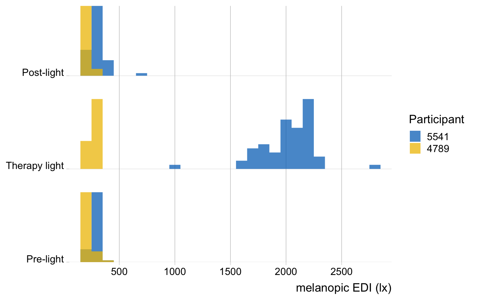

6.2 Table

This section serves to create a fully code-based tabular overview of the data. First, we need to collect the data in the necessary format. Here, one important question arises. Because of the interruptions, no participant has a singular period for all three conditions (pre, light, post). Depending on the LightLogR functions we use, we can either calculate key metrics for all times a certain state is active (by state), or by each episode a certain state is active (by episode). In our case, the by state approach is the better one, but we will highlight both workflows here:

data |>
1  extract_states(state) |>
2  extract_metric(data,
                 mean = mean(MEDI),
                 dose = dose(MEDI, Datetime, epoch = "60s", na.rm = TRUE )) |>
3  summarize_numeric() |>
  select(Id, state, episodes, mean_mean, mean_dose, total_duration) |> 
  drop_na()

1: Condense the dataset to an account of each episode of state (given the grouping by participant). While this is very close to our original state_data it takes the wearable data into account as well.
2: We extract specific metrics from the original dataset with regards to the extracted data. In this case the arithmetic mean (as logarithmic distribution is not really an issue here), and the dose of light.
3: This function not only calculates the average of values within each group (participant and state in this case), but also provide the total duration for each condition.

# A tibble: 8 × 6
# Groups:   Id [2]
  Id    state             episodes mean_mean mean_dose total_duration     
  <fct> <fct>                <int>     <dbl>     <dbl> <Duration>         
1 4789  Pre-light                1      236.    181.   2760s (~46 minutes)
2 4789  Therapy light            2      251.    125.   3360s (~56 minutes)
3 4789  Post-light               1      227.    171.   2700s (~45 minutes)
4 4789  Desk (horizontal)        1      387.      6.45 60s (~1 minutes)   
5 5541  Pre-light                1      273.    210.   2760s (~46 minutes)
6 5541  Therapy light            1     2022.   2056.   3660s (~1.02 hours)
7 5541  Post-light               2      315.    108.   2640s (~44 minutes)
8 5541  Desk (horizontal)        1      331.      5.52 60s (~1 minutes)

Have a special look at the dose. Participant 4789 has an average illuminance of ~250 lx during Therapy light, which lasted for a total of 56 minutes. But the dose only shows ~ 125 lx·h. The reason for that is, because it is not dose, but the mean_dose across all episodes, of which there are two (due to the interruption). We could correct that bei either scaling the dose by episode post-hoc, or by using a manual summary function that takes the duration of individual episodes into account. Instead, we have a different way of getting to the correct outcome by using the durations() function instead of extract_states().

1data_prep <-
data |>
  drop_na(state) |> 
  group_by(state, .add = TRUE)

data_prep |> 
2  durations(MEDI) |>
3  extract_metric(data_prep,
4                 identifying.colname = state,
                 mean = mean(MEDI), 
                 dose = dose(MEDI, Datetime, epoch = "60s", na.rm = TRUE )) |>
  select(Id, state, mean, dose, total_duration = duration)

1: We require a dataset that is also grouped by the state variable
2: Calculate the duration of every state - but only when a value for melanopic EDI is available
3: The function requires the same dataset that was the basis for durations().
4: It further requires an identifying column name for the extraction. In our case, the state column is sufficient

# A tibble: 8 × 5
# Groups:   Id, state [8]
  Id    state              mean    dose total_duration     
  <fct> <fct>             <dbl>   <dbl> <Duration>         
1 4789  Pre-light          236.  181.   2760s (~46 minutes)
2 4789  Therapy light      267.  249.   3360s (~56 minutes)
3 4789  Post-light         227.  171.   2700s (~45 minutes)
4 4789  Desk (horizontal)  387.    6.45 NA                 
5 5541  Pre-light          273.  210.   2760s (~46 minutes)
6 5541  Therapy light     2022. 2056.   3660s (~1.02 hours)
7 5541  Post-light         295.  217.   2640s (~44 minutes)
8 5541  Desk (horizontal)  331.    5.52 NA

Again, have a look at the dose. Participant 4789 has an average illuminance of ~267 lx during Therapy light, which lasted for a total of 56 minutes. The dose is 249 lx·h, which is exactly what you would get by dividing 267lx by 60 minutes times 56 minutes.

Thus we will continue with the by state method and prepare the data for the table

data_tbl_comparison <- 
data_prep |> 
  durations(MEDI) |> 
  extract_metric(data_prep, 
                 identifying.colname = state, 
                 mean = mean(MEDI), 
                 dose = dose(MEDI, Datetime, epoch = "60s", na.rm = TRUE )) |>
  select(Id, state, mean, dose, total_duration = duration) |> 
  mutate(Id = case_when(  
                        Id == "4789" ~ "Control condition", 
                        Id == "5541" ~ "Therapy light"), 
1         across(contains("total_duration"), \(x) replace_na(x, dminutes(1)))
         ) |>
2  pivot_wider(id_cols = state,
              names_from = Id,
              values_from = c(mean, total_duration, dose)) |>
  arrange(state) |> 
  select(1, 2, 4, 6, 3, 5, 7)

1: If there is only a singular datapoint, durations() can not discern its validity duration. Here we manually exchange it for the epoch.
2: By pivoting wider we move from one row per condition and participant to one row per condition.

Then we can produce the table. This next code cells does not contain any LightLogR functions, but simply uses our previous output (data_tbl_comparison) and prints it as a gt table.

data_tbl_comparison |> 
  gt(rowname_col = "state", groupname_col = NULL) |> 
  tab_spanner("Control condition", contains("Control condition")) |> 
  tab_spanner("Therapy lamp", contains("Therapy light", ignore.case = FALSE)) |> 
  cols_label_with(
    fn = \(x) x |> 
               str_remove_all(" |_|Control|condition|Therapy|total|light|No") |> 
               str_to_title()
    ) |> 
  tab_style(locations = cells_column_spanners(1),
            style = cell_text(color = "#EFC000", weight = "bold")
  ) |> 
  tab_style(locations = cells_column_spanners(2),
            style = cell_text(color = "#0073C2", weight = "bold")
  ) |> 
  cols_align("left", columns = state) |> 
  cols_add(
    `Rel. difference` = 
    (`dose_Therapy light`-`dose_Control condition`)/`dose_Control condition`) |> 
  fmt(columns = contains("mean"), 
      fns =  \(x) vec_fmt_number(x, decimals = 0, pattern = "{x} lx")
      ) |> 
  fmt(columns = contains("dose"), 
      fns =  \(x) vec_fmt_number(x, decimals = 0, pattern = "{x} lx·h")
      ) |> 
  fmt_percent(contains("difference"), force_sign = TRUE, decimals = 0) |> 
  gt::cols_width(-state ~ px(100), 
                 state ~ px(150)) |> 
  grand_summary_rows(
    columns = contains("dose"),
    fns = list(label = "Overall", id = "overall", fn = "sum"),
    fmt = contains("dose")~ fmt_number(., decimals = 0, pattern = "{x} lx·h")
  ) |> 
  grand_summary_rows(
    columns = contains("duration"),
    fns = list(label = "Overall", id = "overall", fn = "sum"),
    missing_text = "",
    fmt = ~ fmt_duration(., input_units = "seconds", output_units = "minutes",
                         duration_style = "wide"),
  ) |> 
  gt::grand_summary_rows(
    fns = list(label = "Overall", id = "totals") ~ 
      (sum(`dose_Therapy light`)/sum(`dose_Control condition`)-1),
    fmt = ~ gt::fmt_percent(., decimals = 0, force_sign = TRUE),
    columns = dplyr::contains("difference"),
    missing_text = ""
    ) |> 
  fmt_duration(contains("duration"), 
               input_units = "seconds", 
               output_units = "minutes",
               duration_style = "wide") |> 
  tab_style(locations = list(cells_stub(), 
                             cells_column_labels(),
                             cells_stub_grand_summary()),
            style = cell_text(weight = "bold"))

	Control condition			Therapy lamp			Rel. difference
	Mean	Duration	Dose	Mean	Duration	Dose	Rel. difference
Pre-light	236 lx	46 minutes	181 lx·h	273 lx	46 minutes	210 lx·h	+16%
Therapy light	267 lx	56 minutes	249 lx·h	2,022 lx	61 minutes	2,056 lx·h	+725%
Post-light	227 lx	45 minutes	171 lx·h	295 lx	44 minutes	217 lx·h	+27%
Desk (horizontal)	387 lx	1 minute	6 lx·h	331 lx	1 minute	6 lx·h	−14%
Overall		148 minutes	607 lx·h		152 minutes	2,487 lx·h	+310%

6.3 Plot

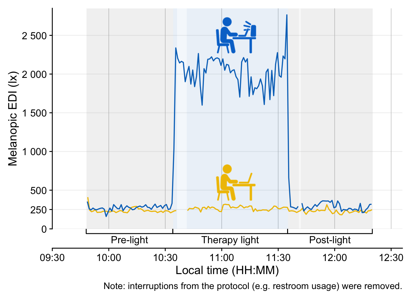
In this section we create two plots of our data, highlighting the differences due to the intervention. The first plot contains a timeline of melanopic EDI, the second the cumulative dose.

We start with a few necessary preparations:

# times set the experimental states
times <- c(9 +48/60, 10 + 34/60, 11 + 35/60, 12 + 20/60)*60*60

# define a protocol axis for plotting
protocol_bracket <- primitive_bracket(
  # Keys determine what is displayed
  key = key_range_manual(start = times[1:3], end = times[2:4], level = 1,
                         name = c("Pre-light", "Therapy light", "Post-light")),
  bracket = "square",
  theme = theme(legend.text = element_text(face = "bold"))
)

#paths to symbols
path_lamp <- "assets/advanced/5541.png"
path_default <- "assets/advanced/4789.png"

#get relevant data for plotting the symbols
symbols <- 
data |> 
  drop_na(state) |> 
  summarize(
    dose(MEDI, Datetime, na.rm = TRUE, as.df = TRUE),
    total_duration = n()*60
  ) |> 
  tibble(
    image = c(path_default, path_lamp),
    y = c(600, 2500),
    x = c(11.125*60*60)
  )

Now we are ready to create the first plot:

data |> 
1  drop_na(state) |>
  filter(state != "Desk (horizontal)") |>
2  gap_handler() |>
3  gg_day(aes_col = fct_rev(Id),
4         geom = "line",
5         facetting = FALSE,
6         y.scale = "identity",
7         x.axis.breaks = hms::hms(hours = seq(0, 24, by = 0.5)),
8         y.axis.breaks = c(0, 250,seq(500, 2500, by = 500))) |>
9  gg_states(state,
            aes_fill = state,
            alpha = 0.05,
            ) +
10  scale_fill_manual(values = c(`Therapy light` = "#0073C2FF")) +
  guides(fill = "none", color = "none", 
11         x = guide_axis_stack(protocol_bracket, "axis")) +
12  coord_cartesian(xlim = c(9.5, 12.6)*60*60,
                  ylim = c(0, 2850), 
                  expand = FALSE) +
13  geom_image(data = symbols, inherit.aes = FALSE,
             aes(image = image, x = x, y = y), size = 0.2, alpha = 1) +
  labs(caption = 
         "Note: interruptions from the protocol (e.g. restroom usage) were removed."
       )

1: Remove all the states that do not belong the experimental protocol
2: Fill in empty observations for the filtered times
3: LightLogR plotting function - we use the reverse coding of participants to get the desired coloring
4: By default gg_day() plots points, this changes it to lines
5: By default, gg_day() creates one panel per day. In this case, we are not interested in identifying the day.
6: By default, gg_day() scales with symlog to include 0 with logarithmic scaling. "identity" simply sets it to a linear scale.
7: By default, gg_day() creates breaks every three hours, here we set it to every half hour.
8: By default, gg_day() sets breaks every 10^ step. Here we set it to steps of 500 lx, but also keeping 250 lx, as that is the base intensity.
9: gg_states() adds the backdrop of states. Try setting ymin and ymax.
10: Ensures that the Therapy light condition has a blue coloring
11: Adds the axis we prepared before
12: Reduce the limits of the plots to areas of interest
13: Adding the symbols

Lastly, we create a cumulative plot. Only the differences compared to above will be highlighted here.

data |> 
  drop_na(state) |>
  filter(state != "Desk (horizontal)") |> 
  mutate(
1    dose = cumsum(MEDI)/60
  ) |> 
  gap_handler() |>
  gg_day(aes_col = fct_rev(Id), geom = "line", facetting = FALSE,
2         y.axis = dose,
         y.scale = "identity",
         x.axis.breaks = hms::hms(hours = seq(0, 24, by = 0.5)),
         y.axis.breaks = c(seq(0, 2500, by = 500))
         ) |> 
  gg_states(state, aes_fill = state, alpha = 0.05) +
  scale_fill_manual(values = c(`Therapy light` = "#0073C2FF")) +
  guides(fill = "none", color = "none", 
         x = guide_axis_stack(protocol_bracket, "axis")) +
  coord_cartesian(xlim = c(9.5, 12.6)*60*60, 
                  ylim = c(0, 2850),
                  expand = FALSE,
                  clip = FALSE
                  ) +
  geom_image(data = symbols, inherit.aes = FALSE,
             aes(image = image,
                 x = 12.48*60*60,
                 y = dose),
             size = 0.15
             ) +
  labs(
    caption = 
      "Note: interruptions from the protocol (e.g. restroom usage) were removed."
    )

1: We calculate a cumulative value from start to end for each participant
2: We set the y.axis variable to dose instead of the default MEDI

7 Conclusion

Congratulations! You have finished this section of the advanced course. If you go back to the homepage, you can select one of the other use cases.