---
title: "Tropical light exposure & health"
author:
- name: "Johannes Zauner"
affiliation: "Technical University of Munich, Germany"
orcid: "0000-0003-2171-4566"
format: live-html
engine: knitr
page-layout: full
toc: true
number-sections: true
date: last-modified
lightbox: true
code-tools: true
code-link: true
webr:
# render-df: gt-interactive
packages:
- LightLogR
- tidyverse
- dplyr
- gt
- melidosData
repos:
- https://tscnlab.r-universe.dev
- https://melidosproject.r-universe.dev
- https://cloud.r-project.org
---
{{< include ./_extensions/r-wasm/live/_knitr.qmd >}}
## Preface
Personal light exposure (PLE) varies strongly between geographic locations, photoperiod, climate, the built environment, culture, and especially dependent on human behaviour. This is important, as PLE is increasingly indicated in not just acute effects, like alertness, mood, and wellbeing, but also longterm mental, metabolic, and cardiovascular health. To support longterm health, recommendations for healthy daytime, evening, and nighttime light have been developed, based on laboratory studies on the so-called non-visual effects of light throughout this century[^1].
[^1]: [Brown et al. (2025)](https://journals.plos.org/plosbiology/article?id=10.1371/journal.pbio.3001571)
Wearable light loogers are used to assess personal light exposure under naturalistic conditions. However, our understanding of PLE is dominated from western, industrialized, high-income countries, and especially limited to how PLE varies in different climates. The [MeLiDos project](https://github.com/MeLiDosProject) captured annotated, high-resolution and multi-country datasets with a harmonized protocol in Sweden, the Netherlands, Germany, Spain, Turkey, Costa Rica, and Ghana (@fig-melidos).
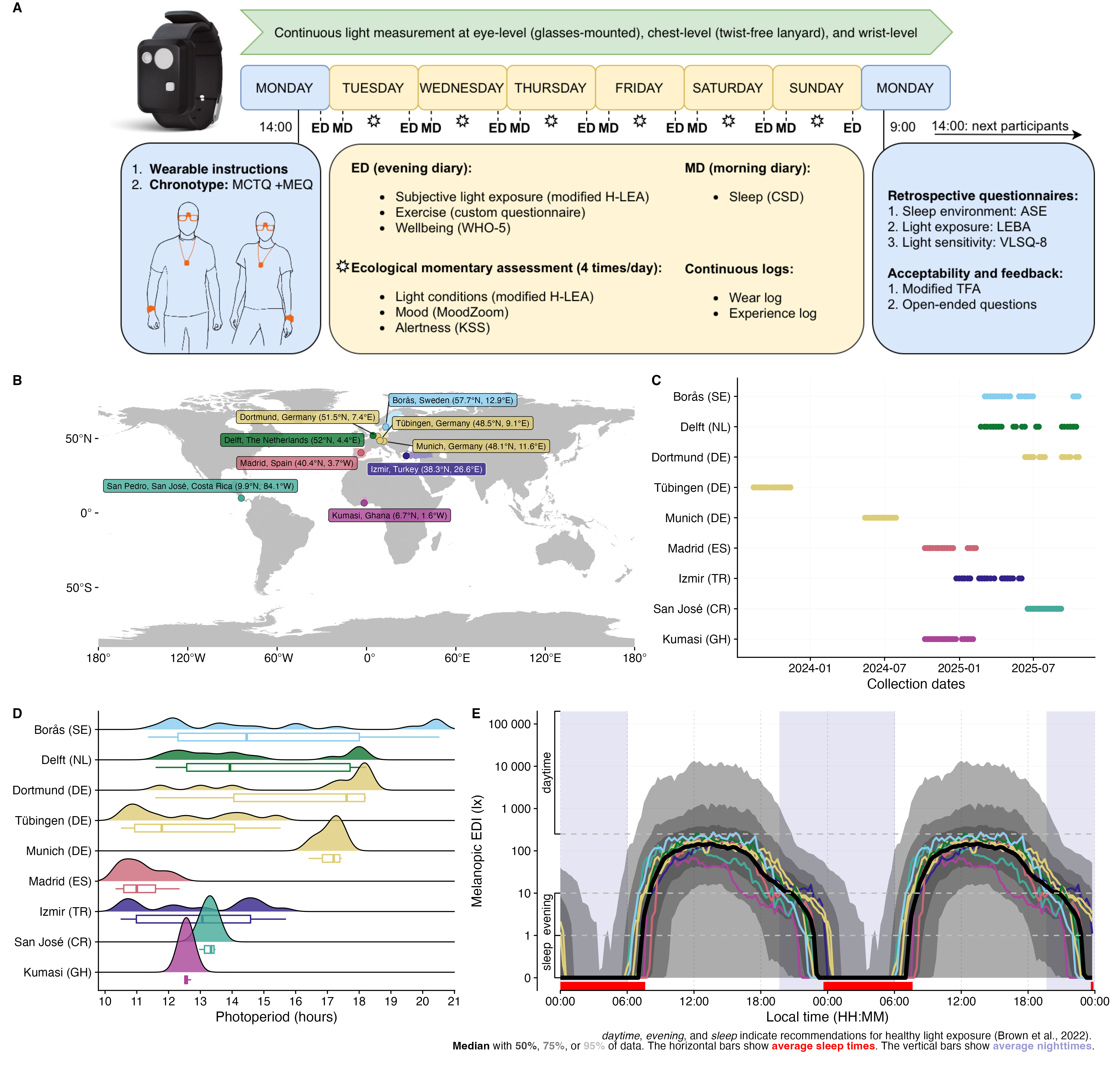{#fig-melidos}
This document uses the [melidosData](https://melidosproject.github.io/melidosData/) R package to load and analyze MeLiDos study data for the `Costa Rica` site. The document has the following goals:
- load chest-level wearable data for `Costa Rica`
- create plots to gain an understanding of exposure patterns
- calculate common exposure metrics
- load sleep-wake data for the same dataset
- merge sleep-wake data with PLE data
- calculate, summarize, and visualize adherence to recommendations for PLE
The analysis uses standardized processing pipelines through the [LightLogR](https://tscnlab.github.io/LightLogR/) package.
`LightLogR` is designed to facilitate the principled import, processing, and visualization of such wearable‑derived data. An accessible entry point to `LightLogR` via a self‑contained analysis script is shown [here](beginner.qmd). Full documentation of `LightLogR`’s features is available on the [documentation page](https://tscnlab.github.io/LightLogR/), including numerous tutorials.
This document assumes general familiarity with the R statistical software, ideally in a data‑science context[^2].
[^2]: If you are new to the R language or want a great introduction to R for data science, we can recommend the free online book [R for Data Science (second edition)](https://r4ds.hadley.nz) by Hadley Wickham, Mine Cetinkaya-Rundel, and Garrett Grolemund.
## How this page works
This document runs a self‑contained version of R **completely in your browser**[^10]. No setup or installation is required.
As soon as as *webR* has finished loading in the background, the **Run Code** button on code cells will become available. You can change the code and execute it either by clicking **Run Code** or by hitting `CTRL+Enter` (Windows) or `CMD+Enter` (MacOS).
Some code lines have commments below. These indicate code-cell line numbers
If you want to see the full analysis without interactive parts, try the [static version](tropical_light_exposure_health.qmd).
[^10]: If you want to know more about `webR` and the `Quarto-live` extension that powers this document, you can visit the [documentation page](https://r-wasm.github.io/quarto-live/)
## Installation
`melidosData` is hosted on [CRAN](https://cran.r-project.org/package=melidosData), which means it can easily be installed from any R console through the following command:
```{webr}
#| eval: false
install.packages("melidosData")
```
After installation, it becomes available for the current session by loading the package. We also require a number of packages. Most are automatically downloaded with `LightLogR`, but need to be loaded separately. Some might have to be installed separately on your local machine.
```{webr}
#| eval: false
library(melidosData) #load the package
library(LightLogR) #load the package
library(tidyverse) #a package for tidy data science
library(gt) #a package for great tables
#the following packages are needed for preview functions:
```
```{webr}
#| include: false
#| autorun: true
# Set a global theme for the background
theme_set(
theme(
panel.background = element_rect(fill = "white", color = NA)
)
)
```
We start by making a decision on the site we want to look at and collect some metadata about it.
```{webr}
site <- "UCR"
melidos_coordinates[[site]]
melidos_colors[[site]]
melidos_cities[[site]]
melidos_countries[[site]]
melidos_tzs[[site]]
```
Want to use a different site? Just switch the Institution name in the code cell above
| Institution (site Abbr.) | City | Country | Repository | DOI |
|----------|----------|-------------|--------------------------|---------------------|
| `KNUST` | Kumasi | Ghana | [AkuffoEtAl_Dataset_2025](https://github.com/MeLiDosProject/AkuffoEtAl_Dataset_2025) | 10.5281/zenodo.15576731 |
| `UCR` | San José | Costa Rica | [Sancho-SalasEtAl_Dataset_2025](https://github.com/MeLiDosProject/Sancho-SalasEtAl_Dataset_2025) | 10.5281/zenodo.17289456 |
| `IZTECH` | Izmir | Turkey | [DidikogluEtAl_Dataset_2025](https://github.com/MeLiDosProject/DidikogluEtAl_Dataset_2025) | 10.5281/zenodo.16568109 |
| `FUSPCEU` | Madrid | Spain | [BaezaEtAl_Dataset_2025](https://github.com/MeLiDosProject/BaezaEtAl_Dataset_2025) | 10.5281/zenodo.16834951 |
| `TUM` | Munich | Germany | [HildenEtAl_Dataset_2025](https://github.com/MeLiDosProject/HildenEtAl_Dataset_2025) | 10.5281/zenodo.16893901 |
| `MPI` | Tübingen | Germany | [GuidolinEtAl_Dataset_2025](https://github.com/MeLiDosProject/GuidolinEtAl_Dataset_2025) | 10.5281/zenodo.16895188 |
| `BAUA` | Dortmund | Germany | [BroszioEtAl_Dataset_2025](https://github.com/MeLiDosProject/BroszioEtAl_Dataset_2025) | 10.5281/zenodo.18111232 |
| `THUAS` | Delft | The Netherlands | [AertsEtAl_Dataset_2025](https://github.com/MeLiDosProject/AertsEtAl_Dataset_2025) | 10.5281/zenodo.17979893 |
| `RISE` | Borås | Sweden | [NilssonTengelinEtAl_Dataset_2026](https://github.com/MeLiDosProject/NilssonTengelinEtAl_Dataset_2026) | 10.5281/zenodo.18925834 |
: Overview of the available sites in the package
## Load and visualize light exposure data for `Costa Rica`
The `load_data()` function loads pre-processed data from the *MeLiDos* project. The `site` argument can be set to one or multiple sites. In our case, `UCR` loads data collected by the *University of Costa Rica*. To reduce data complexity, we use 1-minute aggregated data.
```{webr}
data <- load_data("light_chest_1minute", site = site)
#try setting "light_glasses_1minute", or switch to a different site instead
data |> head()
```
We can explore this dataset in several, low-effort ways.
```{webr}
#| fig-width: 10
#| fig-height: 5
data |>
gg_overview() + #create the overview plot
theme_sub_axis_y(text = element_blank()) #remove y-axis text
```
```{webr}
data |>
summary_overview() |> #calculate overview stats
gt() |> sub_missing() |> #show as table
tab_header(
paste0("Dataset overview for ",
melidos_cities[[site]], ", ",
melidos_countries[[site]])
)
```
```{webr}
#| fig-width: 8
#| fig-height: 7
data |>
sample_groups(5) |> #select 5 groups (participants)
aggregate_Datetime("30 mins", type = "floor") |> #condense data to 30-minute intervals
gg_days() |> #create timeline plot
gg_photoperiod(melidos_coordinates[[site]]) #add photoperiod information
```
```{webr}
data |>
ungroup() |> #remove by-participant grouping
aggregate_Date(unit = "30 mins") |> #condense data to 1 day of 30-minute intervals
gg_doubleplot(fill = melidos_colors[[site]]) |> #create double plot
gg_photoperiod(melidos_coordinates[[site]]) #add photoperiod information
```
## Calculate common exposure metrics
`LightLogR` has a summary function that calculates many common metrics and shows how they are distributed within the dataset.
The following section cannot be run in the interactive session, thus the output will be directly shown in @tbl-metrics.
```{webr}
#| eval: false
data |>
summary_table( #summary table function
melidos_coordinates[[site]], #provide coordinates for photoperiod calculation
location = melidos_cities[[site]], #provide a label for location
site = melidos_countries[[site]], #provide a label for site
color = melidos_colors[[site]] #provide a color for histogram generation
)
```
:::{.panel-tabset}
### Chest-level
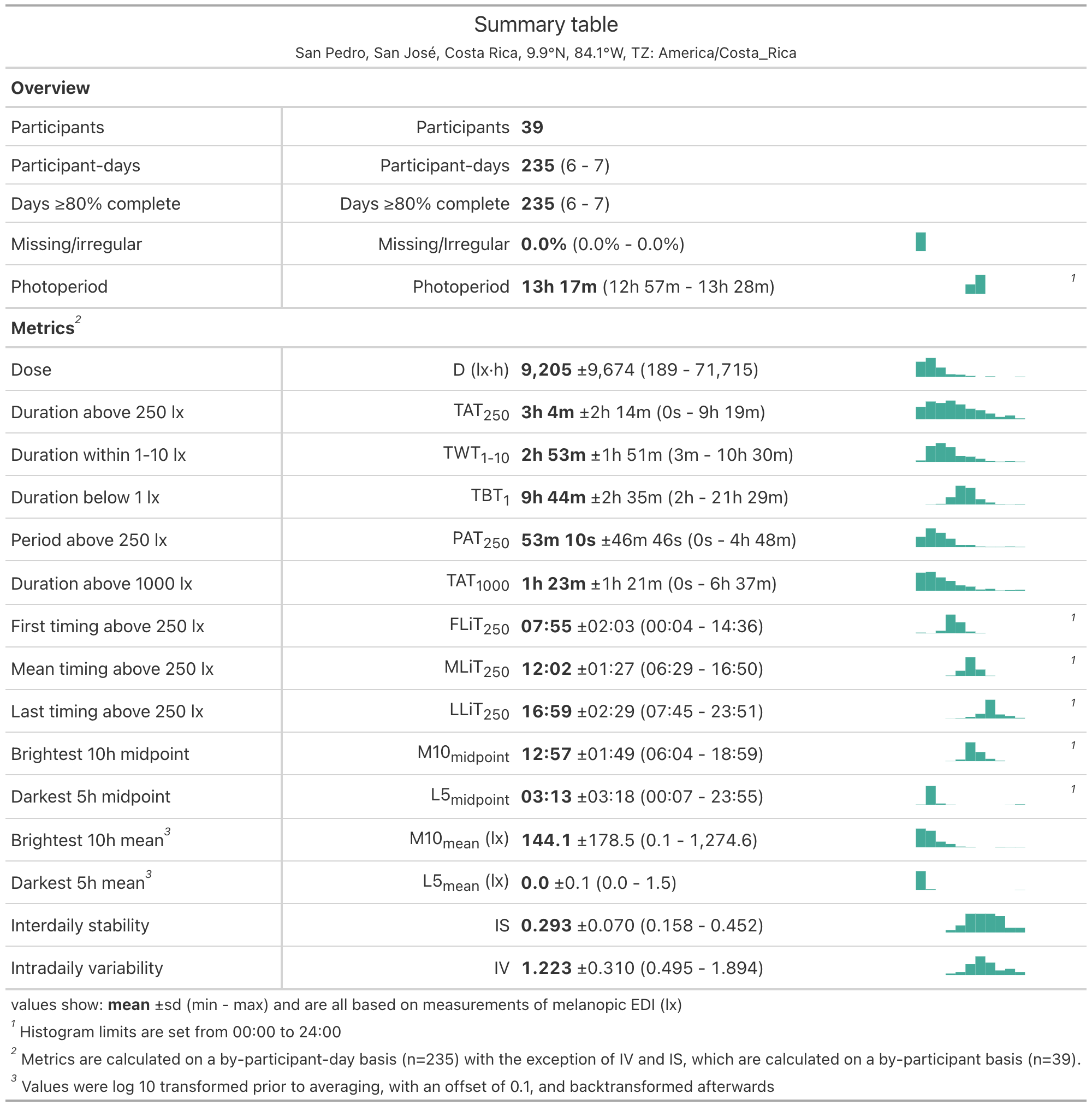{#tbl-metrics}
### Glasses-level
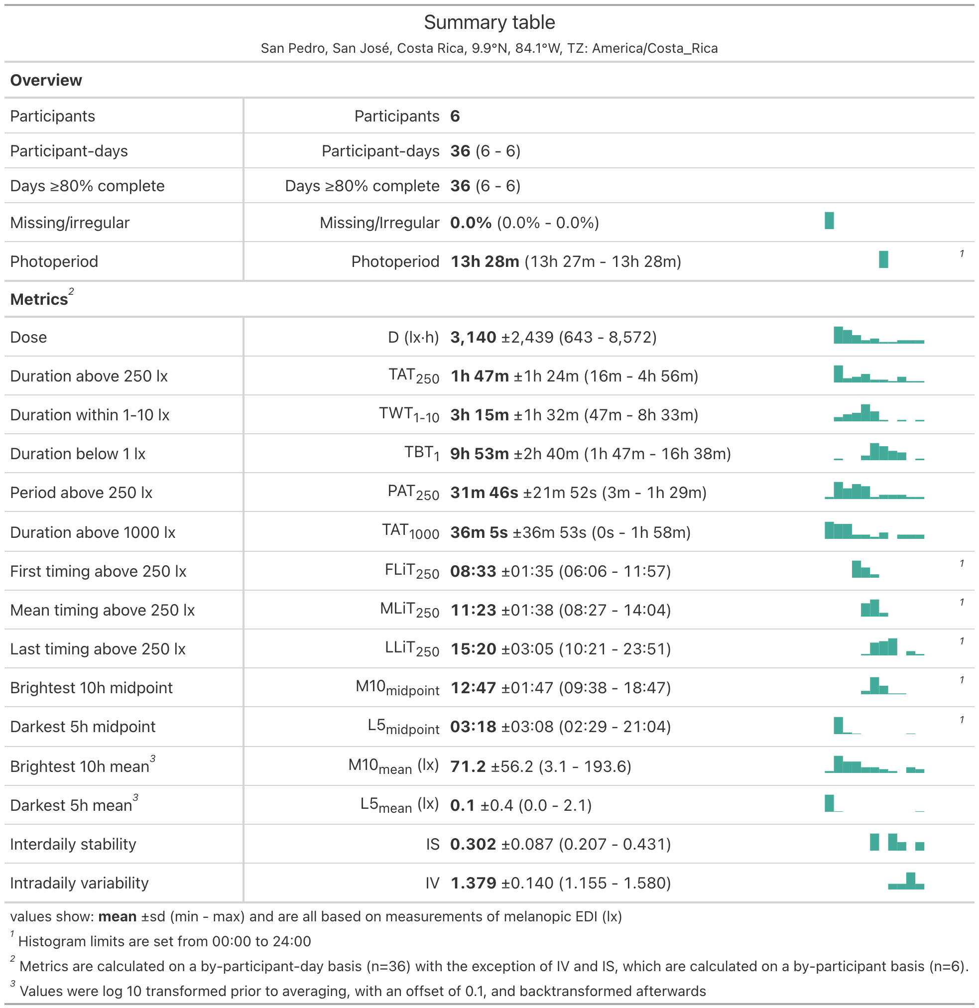{#tbl-metrics_glasses}
:::
## Load and merge sleep-wake data with light exposure data
We start by loading `sleepdiaries` data. Because we only want to check for data when devices were worn, we also load the `wearlog` information.
```{webr}
sleepdata <- load_data("sleepdiaries", site = site)
wearlog <- load_data("wearlog", site = site)
```
We can quickly check what information is available in both datasets with the `extract_labels()` function.
```{webr}
sleepdata |> extract_labels() |> head()
wearlog |> extract_labels() |> head()
```
In the next step, we prepare the sleepdiary data by selecting a subset containing the participant `ID`, as well as the time when participants prepared to sleep (`sleepprep`) and when the woke (`wake`). Because we are not only interested in labelling sleep periods, but also the in-between wake periods, we pivot the data to a longer form and transform them to intervals. Based on those sleep and wake intervals, we assign states according to Brown et al. (day, evening, night).
```{webr}
sleepdata <-
sleepdata |>
select(Id, sleep = sleepprep, wake) |> #subset of the sleepdiaries
group_by(Id) |> #group by participant
pivot_longer(-Id, names_to = "sleep", values_to = "Datetime") |> #reshape to one row per state
sc2interval(Statechange.colname = sleep, starting.state = "wake") |> #intervals (with max length) instead of timestamps
sleep_int2Brown(sleep.state = "sleep", Brown.day = "wake", #Brown et al. intervals
Brown.evening = "pre-sleep", Brown.night = "sleep") |> #Brown et al. intervals
mutate(sleep = case_when(is.na(sleep) & State.Brown == "pre-sleep" ~ "wake", #fill in values for pre-sleep
.default = sleep))
names(sleepdata)
```
The transformed sleep data, as well as photoperiod information and wear states get added to the light exposure data.
```{webr}
data <-
data |>
select(Id, Datetime, MEDI) |> #subset of light data
add_photoperiod(melidos_coordinates[[site]]) |> #add photoperiod information
add_states(sleepdata, start = Interval, end = Interval) |> #add sleep information
add_states(wearlog |> select(Id, start, end, wear = state)) #add wear information
names(data)
```
Next, we want to remove instances from the Brown states when the device was not worn during the day or evening.
```{webr}
#Remove non-wear data during wake or pre-sleep
data <-
data |>
mutate(
State.Brown = case_when(
wear == "off" & sleep != "sleep" ~ NA,
.default = State.Brown
)
)
print("executed")
```
We can visualize this combined dataset by stacking several of the previous functions and adding the state information on top.
```{webr}
#| fig-width: 10
#| fig-height: 5
data |>
sample_groups(3) |> #select three participants
aggregate_Datetime("30 mins", type = "floor") |> #aggregate to 30-minute bins
mutate(State.Brown = #order factor labels (for coloring)
factor(State.Brown, levels = c("wake", "pre-sleep", "sleep"))) |>
gg_days() |> #create base-plot
gg_photoperiod() |> #add photoperiod information
gg_states(State.Brown, #add state information
aes_fill = State.Brown, #fill by state
ymax = 0, alpha = 1 #only create a small band
) +
labs(fill = "State") # adjust legend label
```
## Adherence to Brown et al. recommendations
The first step is to check whether the melanopic EDI were satisfactory at a given moment through the `Brown2reference()` function.
```{webr}
data <-
data |>
Brown2reference(Brown.day = "wake", #check whether melEDI are ok
Brown.evening = "pre-sleep",
Brown.night = "sleep")
names(data)
```
Based on the previous figure, we can add information on whether a given timepoint was adherent to the recommendations.
```{webr}
#| fig-width: 10
#| fig-height: 5
data |>
sample_groups(3) |> #sample 3 groups
aggregate_Datetime("30 mins", type = "floor") |> #30-minute intervals
mutate(State.Brown = #create a factor and add an Unknown type
factor(State.Brown |> replace_na("Unknown"),
levels = c("wake", "pre-sleep", "sleep", "Unknown")),
Reference.check = case_when( #set names for adherence
Reference.check ~ "Good",
!Reference.check ~ "Bad",
.default = "Unknown"
)) |>
gg_days( #create the base plot
jco_color = FALSE, #do not use default fill scale
geom = "ribbon", #use a ribbon geom
aes_fill = State.Brown, #fill the ribbon by state
group = consecutive_id(State.Brown) #group those fills by occurances of state
) |>
gg_photoperiod() |> #add photoperiod
gg_states(Reference.check, #add state information of adherance
aes_fill = Reference.check, #fill by adherence
ymax = 0, alpha = 1, #only a small band
on.top = TRUE, #put band on top
) +
geom_line() + #add a line on top of everything
labs(fill = "State") + #adjust legend label
scale_fill_manual(values = c(wake = "skyblue3", `pre-sleep` = "gold",
sleep = "grey", Bad = "red", Good = "green3",
Unknown = "white")) #manual scale
```
We can also highlight when in the day recommendation is highest and lowest.
```{webr}
data |>
add_Time_col() |> #add a time column
drop_na(Reference.check) |> #remove instances where state is unknown
ggplot(aes(x = Time)) + #create a plot across time
geom_density(aes(fill = Reference.check), position = "fill") + #with scaled stacked densities
scale_fill_manual(values = c("red2", "green3")) + #manual scale
labs(fill = "Within recommendations") #adjust legend label
```
Finally, we calculate exact adherance percentages across states...
```{webr}
adherence_summary <-
data |>
group_by(State.Brown) |> #group data by Brown state
durations(Reference.check, #calculate the length for each group
show.missing = TRUE, #show where data is missing
FALSE.as.NA = TRUE) |> #regard a FALSE in the data as missing
ungroup() |> #remove grouping
mutate(across(duration:missing, \(x) x/total), #calculate percentages
of.total = (total/sum(total)) |> as.numeric(), #calculate percentages
duration = case_when(duration == 0 ~ NA, .default = duration)) |> #set missing
rename(adherence = duration,
duration = total) |> #rename
select(-missing) #remove unneeded column
adherence_summary
```
...and add a summary row
```{webr}
adherence_summary <-
adherence_summary |>
drop_na() |>
summarize( #calculate summary row:
State.Brown = "Overall",
adherence = (adherence*of.total) |> sum(),
duration = sum(duration) |> as.duration(),
of.total = sum(of.total),
adherence = adherence/of.total
) |>
rbind(adherence_summary) #add the summary row to the detailed table
adherence_summary
```
In the final step, we bring this table into a nice layout.
```{webr}
adherence_summary |>
gt() |>
fmt_percent(c(adherence, of.total), decimals = 1) |> #format as percent
sub_missing(missing_text = "Unkown") |> #rename missing entries
cols_label_with(fn = \(x) str_replace(x, "\\.", " ") |> str_to_title()) |> #tranform labels
tab_style( #show some cells bold
cell_text(weight = "bold"),
list(cells_column_labels(), cells_body(1))
) |>
tab_style( #show a highlight for the summary row
cell_fill("lightgrey"),
cells_body(rows = 1)
) |>
fmt_duration(duration, input_units = "seconds", output_units = "weeks") |> #format as duration
tab_header("Adherence to recommendations for healthy lighting", # add a header
subtitle =
paste0(melidos_cities[[site]], melidos_countries[[site]], sep = ", ")
)
```


