---
title: "Analysis of human visual experience data"
author:
- name: "Johannes Zauner"
id: JZ
affiliation:
- Technical University of Munich, Germany
- Max Planck Institute for Biological Cybernetics, Germany
orcid: "0000-0003-2171-4566"
corresponding: true
email: johannes.zauner@tum.de
- name: "Aaron Nicholls"
id: AN
affiliation: "Reality Labs Research, USA"
orcid: "0009-0001-6683-6826"
- name: "Lisa A. Ostrin"
id: LAO
affiliation: "University of Houston College of Optometry, USA"
orcid: "0000-0001-8675-1478"
- name: "Manuel Spitschan"
id: MS
affiliation:
- Technical University of Munich, Germany
- Max Planck Institute for Biological Cybernetics, Germany
- Technical University of Munich, Institute for Advanced Study (TUM-IAS), Germany
orcid: "0000-0002-8572-9268"
abstract: >
Exposure to the optical environment — often referred to as *visual experience* — profoundly influences human physiology and behavior across multiple time scales. In controlled laboratory settings, stimuli can be held constant or manipulated parametrically. However, such exposures rarely replicate real-world conditions, which are inherently complex and dynamic, generating high-dimensional datasets that demand rigorous and flexible analysis strategies. This tutorial presents an analysis pipeline for visual experience datasets, with a focus on reproducible workflows for human chronobiology and myopia research. Light exposure and its retinal encoding affect human physiology and behavior across multiple time scales. Here we provide step-by-step instructions for importing, visualizing, and processing viewing distance and light exposure data. This includes time-series analyses for working distance, biologically relevant light metrics, and spectral characteristics. The tasks are standardized through the open-source R package [**LightLogR**](https://tscnlab.github.io/LightLogR/). By leveraging a modular approach, the tutorial supports researchers in building flexible and robust pipelines that accommodate diverse experimental paradigms and measurement systems.
keywords:
- wearable
- light logging
- viewing-distance
- visual experience
- metrics
- circadian
- myopia
- risk factors
- spectral analysis
- open-source
- reproducibility
funding: "JZs position is funded by MeLiDos, The project (22NRM05 MeLiDos) has received funding from the European Partnership on Metrology, co-financed from the European Union’s Horizon Europe Research and Innovation Programme and by the Participating States. Views and opinions expressed are however those of the author(s) only and do not necessarily reflect those of the European Union or EURAMET. Neither the European Union nor the granting authority can be held responsible for them. JZ, LAO, and MS received funding from Reality Labs Research."
format:
html:
toc: true
toc-depth: 3
toc-location: right
number-sections: true
code-link: true
code-tools: true
grid:
body-width: 850px
html-math-method:
method: mathjax
url: "https://cdnjs.cloudflare.com/ajax/libs/mathjax/2.7.9/latest.js?config=TeX-MML-AM_CHTML"
doi: 10.5281/zenodo.16566014
bibliography: references.bib
lightbox: true
execute:
echo: true
---
## Introduction
{width="40%"}
Exposure to the optical environment — often referred to as *visual experience* — profoundly influences human physiology and behavior across multiple time scales. Two notable examples, from distinct research domains, can be understood through a common retinally-referenced framework.
The first example relates to the non-visual effects of light on human circadian and neuroendocrine physiology. The light–dark cycle entrains the circadian clock, and light exposure at night suppresses melatonin production [@Brown2022PLoSBiol; @Blume2019Somnologie]. The second example concerns the influence of visual experience on ocular development, particularly myopia. Time spent outdoors — which features distinct optical environments — has been consistently associated with protective effects on ocular growth and health outcomes [@DahlmannNoor2025GraefesArchClinExpOphthal].
In controlled laboratory settings, light exposure can be held constant or manipulated parametrically. In contrast, real-world conditions are inherently complex and dynamic, and cannot be captured by single spot measurements. As people move in and between spaces (indoors and outdoors) and move their body, head, and eyes, exposure to the optical environment varies significantly [@Webler2019CurrOpinBehavSci] and is modulated by behavior [@Biller2024CommunPsychol]. Wearable devices for measuring light exposure have thus emerged as vital tools to capture the ecological visual experience. These tools generate high-dimensional datasets that demand rigorous and flexible analysis strategies.
Starting in the 1980s [@Okudaira1983AmJPhysiol], technology to measure optical exposure has matured, with miniaturized illuminance sensors now (in 2025) very common in consumer wearables [@vanDuijnhoven2025BuildEnviron]. In research, several devices are available that differ in functionality, ranging from small pins measuring ambient illuminance [@Mohamed2021OptExpress] to head-mounted multi-modal devices capturing nearly all relevant aspects of visual experience [@Gibaldi2024TranslVisSciTechnol]. Increased capabilities in wearables bring complex, dense datasets. These go hand-in-hand with a proliferation of metrics, as highlighted by recent review papers in both circadian and myopia research [@Honekopp2023ClinOphthalmol; @Hartmeyer2023LightResTechnol].
At present, the analysis processes to derive metrics are often implemented on a per-laboratory or even per-researcher basis. This fragmentation is a potential source of errors and inconsistencies between studies, consumes considerable researcher time [@Hartmeyer2022LightResTechnol], and these bespoke processes and formats hinder harmonization or meta-analysis across multiple studies. It is very common that more time is spent preparing data than gaining insights through rigorous statistical analysis. These preparation tasks are best handled, or at least facilitated, by standardized, transparent, community-based analysis pipelines [@Zauner2024PLOSONE].
In circadian research, the R package LightLogR was developed to address this need [@Zauner2025JOpenSourceSoftw]. LightLogR is an open-source, MIT-licensed, community-driven package specifically designed for data from wearable light loggers and optical radiation dosimeters. It contains functions to calculate over sixty different metrics used in the field [@Hartmeyer2023LightResTechnol]. The package functions come with light-related defaults, but they remain fundamentally agnostic to modality. As a result, parameters like viewing distance and light spectra, both highly relevant to myopia research [@Honekopp2023ClinOphthalmol], can easily be handled.
In this article, we demonstrate that LightLogR’s analysis pipelines and metric functions apply broadly across the field of visual experience research, not just to circadian rhythms and chronobiology. Our approach is modular and extensible, allowing researchers to adapt it to a variety of devices and research questions. Emphasis is placed on clarity, transparency, and reproducibility, aligning with best practices in scientific computing and open science. We use example data from two devices (worn by different individuals and at different times) to showcase the LightLogR workflow with metrics relevant to myopia research, covering working distance, (day)light exposure, and spectral analysis. Readers are encouraged to recreate the analysis using the provided code. All necessary data and code are openly available in the [GitHub repository](https://github.com/tscnlab/ZaunerEtAl_JVis_2026).
::: callout-tip
### Scope
This article focuses on workflows for deriving condensed metrics from time-series data collected with wearable devices in the visual-experience domain. Specifically, we address illuminance, viewing distance, and spectral irradiance. Example datasets from two types of wearable devices are used for illustration.
Many relevant considerations arise when collecting data with wearable devices. This article covers only a subset of these. In particular, it does not address:
- device selection (see, e.g., [@vanDuijnhoven2025BuildEnviron; @Zauner2025LightResTech; @Zauner2026spechelper])
- measurement accuracy or device calibration
- auxiliary data such as sleep/wake information (see, e.g., [@zauner2026; @Guidolin2026])
More information on those aspects can be found in the [*Technical guide for wearable optical radiation dosimetry and visual experience assessment*](https://doi.org/10.17617/6xca-cg59) [@zauner2025].
To demonstrate the workflows, this article uses expert-informed definitions of metrics and metric parameters (see, e.g., @tbl-one, @tbl-two, and the non-wear detection rules based on activity data described in [Supplement 1](supplement.qmd)). These definitions and thresholds should not be interpreted as universal standards, nor are they hard-coded into the software package. For any application, parameter choices must be tailored to the research domain, study context and design, and the specifications of the wearable device. The demonstrated software supports this expressly.
Further, the article is split up in the main analysis part, where all metrics are calculated, and the [Supplement 1](supplement.qmd), where data is imported, screened, and prepared. Thus, the reader is referred to [Supplement 1](supplement.qmd) for all aspects regarding data formats, preparation steps, and handling of gaps, i.e., missing data.
Lastly, the example data used in the article do not stem from a controlled experimental data collection but consist of data gathered in an ecological setting without a fixed protocol. Given the substantial interindividual differences in visual experience metrics, and because the analyses focus on one participant at a time, the reported results should be interpreted as illustrative rather than representative of typical or population-level values.
:::
## Methods and materials
### Software
This tutorial was built with `Quarto`, an open-source scientific and technical publishing system that integrates text, code, and code output into a single document. The source code to reproduce all results is included and accessible via the Quarto document's `code tool` menu. All analyses were conducted in R (version 4.5.0, "How About a Twenty-Six") using `LightLogR` (version 0.10.0 "High noon"). We also used the `tidyverse` suite (version 2.0.0) for data manipulation (which LightLogR follows in its design), and the `gt` package (version 1.1.0) for generating summary tables. A comprehensive overview of the R computing environment is provided in the session info (see [Session info](#sessioninfo) section).
### Metric selection and definitions
In March 2025, two workshops with myopia researchers — initiated by the Research Data Alliance (RDA) Working Group on Optical Radiation Exposure and Visual Experience Data — focused on current needs and future opportunities in data analysis, including the development and standardization of metrics. Based on expert input from these workshops, the authors of this tutorial compiled a list of visual experience metrics, shown in @tbl-one. These include many currently used metrics and definitions [@Wen2020bjophthalmol; @Wen2019TransVisSciTech; @Bhandari2020OphthalmicPhysiolOpt; @Williams2019Scientificreports], as well as new metrics enabled by spectrally-resolved measurements. While they are not derived by a formal consensus process, they are expert-informed and used in current scientific research, and thus will serve as example-definitions for metrics and thresholds throughout this article.
{{< include _Table1.qmd >}}
@tbl-two provides definitions for the terms used in @tbl-one. Note that specific definitions may vary depending on the research question or device capabilities.
{{< include _Table2.qmd >}}
It should be noted that although daylight levels can far exceed the thresholds defined in @tbl-two - and may reach or even exceed 10\^5 lux - empirical daylight levels measured at eye level are much lower, typically around 10\^3 lux, especially when considering aggregated time-series data over minutes to hours.
### Devices {#sec-devices}
Data from two wearable devices are used in this analysis:
- `Clouclip`: A wearable device that measures viewing distance and ambient light simultaneously [Glasson Technology Co., Ltd, Hangzhou, China; @Wen2021ActaOphtalmol; @Wen2020bjophthalmol; @Bhandari2020OphthalmicPhysiolOpt]. The Clouclip provides a simple data output with only distance (working distance, in centimeters) and illuminance (ambient light, in lux). Data in our example were recorded at 5-second intervals. Approximately one week of data (\~120,960 observations) is about 2-4 MB in size. For the `Clouclip` device, the dataset was obtained in November 2020 from a 30-year-old male graduate student in Texas, United States, and was previously presented as part of a published study [@bhandari2021]. The light exposure profile reflects relatively limited time outdoors, which is consistent with patterns reported in individuals engaged in intensive academic training and the pandemic during 2020.
- `Visual Environment Evaluation Tool` (VEET): A head-mounted multi-modal device that logs multiple data streams [Reality Labs Research, Menlo Park, CA, USA; @Sah2025OphtalmicPhysiolOpt; @Sullivan2024]. The VEET dataset used here contains simultaneous measurements of distance (via a time-of-flight sensor), ambient light (illuminance), activity (accelerometer & gyroscope), and spectral irradiance (multi-channel light sensor). Data were recorded at 2-second intervals, yielding a very dense dataset (\~270 MB per week). For the `VEET` device, the dataset comes from pilot data collection of a researcher in Texas, United States, under naturalistic conditions in June 2024 (light and distance) and June 2025 (spectral data). The researcher was working in a typical office building with limited daylight availability during office hours and limited time outdoors overall.
The distribution of light exposure in both datasets is typical for indoor and partial outdoor times and is discussed further at the beginning of the Results section for light exposure.
### Data processing summary
The [Results](#results) section uses imported and pre-processed data from the two devices to calculate metrics. [Supplement 1](supplement.qmd) contains the annotated code and description for the steps involved, which are summarized as follows, and as shown in @fig-fc_supplement. Please refer to the supplement for details.
{{< include _flowchart_supplement.qmd >}}
**Data import:** We imported raw data from the `Clouclip` and `VEET` devices using LightLogR’s built-in import functions, which automatically handle device-specific formats and idiosyncrasies.
The `Clouclip` export file (provided as a tab-delimited text file) contains timestamped records of distance (cm) and illuminance (lux). LightLogR’s `import$Clouclip` function reads this file, after specifying the device’s recording timezone, and converts device-specific sentinel codes into proper missing values. For instance, the Clouclip uses special numeric codes to indicate when it is in “sleep mode” or when a reading is out of the sensor’s range, rather than recording a normal value. LightLogR identifies `-1` (for both distance and lux) as indicating the device’s sleep mode and `204` (for distance) as indicating the object was beyond the measurable range, replacing these with `NA` and logging their status in separate columns. The import routine also provides an initial summary of the dataset, including start and end times and any irregular sampling intervals or gaps. The dataset contained substantial values above the sensible range of 120 cm distance measurement [@Bhandari2020OphthalmicPhysiolOpt], which is why these measurements were set to `NA`, with an identifier of these cases in `Dis_status`.
For the `VEET` device, data were provided as CSV logs (zipped on Github, due to size). We focused on the ambient light sensor modality first. Using `import$VEET(..., modality = "ALS")`, we extracted the illuminance (`Lux`) data stream and its timestamps. The raw VEET data similarly contains irregular intervals and can contain missing periods (e.g., if the device stopped recording or was reset); the import summary flags these issues.
Besides the `Clouclip` and `VEET`, LightLogR 0.10.0 contains import functions for 18 more wearable devices. The package further supports versioning due to evolving data formats, and includes documentation for both [code-based](https://tscnlab.github.io/LightLogR/reference/import_adjustment.html) and [code-less](https://tscnlab.github.io/LightLogR/articles/Import.html#from-which-devices-can-i-import-data) additions of new device import-functions.
**Irregular intervals, gaps, non-wear times:** Both datasets showed irregular timing and missing data, i.e., gaps. Irregular data means that some observations did not align to the nominal sampling interval (e.g., slight timing drift or pauses in recording). For the `Clouclip` 5-second data, we detected irregular timestamps on most days. Handling such irregularities is important because many downstream analyses assume a regular time series. We evaluated strategies to address this, including:
- Removing an initial portion of data if irregularities occur mainly during device start-up.
- Rounding all timestamps to the nearest regular interval (5 s in this case). This is only feasible if no duplicate timestamps are created
- Aggregating to a coarser time interval (with some loss of temporal resolution). It would also be possible to aggregate to the main interval, in case there are duplicate timestamps from rounding.
Based on the import summary and visual inspection of the time gaps, we chose to round the observation times to the nearest 5-second mark, as this addressed the minor offsets without significant data loss. No duplicate time stamps arose. After rounding timestamps, we added an explicit date column for convenient grouping by day.
We then generated a summary of missing data for each day. Implicit gaps (intervals where the device should have recorded data but did not) were converted into explicit missing entries using LightLogR’s gap-handling functions. We also removed days that had very little data to focus on days with substantial wear time. In our `Clouclip` example, days with less than one hour of recordings were dropped. This threshold should be adjusted based on how much complete days matter for a given analysis at hand. E.g., in circadian science, the metrics of *interdaily stability* and *intradaily variation* require measurements for each hour of the day. As we are mostly using the `Clouclip` data for its distance recordings, even short periods are useful.
After these preprocessing steps, the `Clouclip` dataset had no irregular timestamps remaining and contained explicit markers for all periods of missing data (e.g., times when the device was off or not worn). The distance and illuminance values were now ready for metric calculations. Because the device was put in `sleep mode` when not worn, there are no measurements during non-wear times.
The `VEET` illuminance data underwent a similar cleaning procedure. To make the `VEET`’s 2-second illuminance data more comparable to the `Clouclip`’s and to reduce computational load, we aggregated the illuminance time series to 5-second intervals. Aggregation was performed with the arithmetic mean of values in a 5-second bin. We then inserted explicit missing entries for each whole day and removed days with more than one hour of missing illuminance data. After cleaning, six days of `VEET` illuminance data with good coverage remained for analysis (see [Supplement 1](supplement.qmd) for details).
Finally, for spectral analysis, we imported the `VEET`’s spectral sensor modality, and, for the distance analysis, the time-of-flight modality. This required additional processing: the raw spectral data consists of counts from nine wavelength-specific channels (approximately 415 nm through 940 nm, unequally spaced between 30 and 50 nm, plus one broadband clear channel covering the whole range of individual channels, another broadband channel for flicker detection, and a dark channel) along with a sensor gain setting. We aggregated the spectral data to 5-minute intervals to focus on broader trends and reduce data volume. Each channel’s counts were normalized by the appropriate gain. Using a calibration matrix provided by the manufacturer (specific to the spectral sensor model), we reconstructed full spectral power distributions for each 5-minute interval. The end result is a list-column in the dataset where each entry is the estimated spectral irradiance across wavelengths for that time interval. Detailed spectral preprocessing steps, including the calibration and normalization, are provided in the [Supplement 1](supplement.qmd). After spectral reconstruction, the dataset was ready for calculating example spectrum-based metrics.
Similarly, the time-of-flight modality contains 256 values per observation, encoding an 8x8 grid of distance and confidence measurements for up to two objects (8x8 grid, times two objects, times distance + confidence column for each object and grid point -\> 256 values). For computational reasons, only the first object was kept. These data were pivoted into a long format, where each row contains the distance and confidence data for a given position in the grid and a given datetime. After pivoting and converting grid positions into a deviation angle from central view, the dataset was ready to be used for distance analysis.
Because the `VEET` devices record even when not worn, a non-wear detection using the devices' actigraphy modality was implemented. This process used the standard deviation of a linear motion sensor in a 5-minute bin with a visually derived threshold to separate wear from non-wear time. Measurements of illuminance and distance were consequently removed during the calculated non-wear times.
This tutorial will start by importing a `Clouclip` dataset and providing an overview of the data. The `Clouclip` export is considerably simpler compared to the `VEET` export, only containing `Distance` and `Illuminance` measurements. The `VEET` dataset will be imported later for the spectrum related metrics.
```{r}
#| label: setup
#| output: false
#| filename: Load libraries and preprocessed data
library(LightLogR)
library(tidyverse)
library(gt)
library(patchwork)
load("data/cleaned/data.RData")
```
```{r}
#| filename: Store coordinates of data collection
coordinates <- c(29.75, -95.36) #<1>
```
1. Coordinates for Houston, Texas; coordinates are important to calculate and visualize photoperiods later
## Results {#results}
@fig-fc_main shows an overview of the covered workflows in the results section.
{{< include _flowchart_main.qmd >}}
### Distance
We first examine metrics related to viewing distance, using the processed `Clouclip` dataset. Many distance-based metrics are computed for each day and then averaged over weekdays, weekends, or across all days. To facilitate this, we define a helper function that will take daily metric values and calculate the mean values for weekdays, weekends, and the overall daily average:
```{r}
#| filename: Define helper function to_mean_daily()
to_mean_daily <- function(data, prefix = "average_") {
data |>
ungroup(Date) |> #<1>
mean_daily(prefix = prefix) |> # <2>
rename_with(.fn = \(x) str_replace_all(x,"_"," ")) |> # <3>
gt() # <4>
}
```
1. Ungroup by days
2. Calculate the averages per grouping
3. Remove underscores in names
4. Format as a gt table for display
#### Total wear time daily
*Total wear time daily* refers to the amount of time the device was actively collecting distance data each day (i.e. the time the device was worn and operational). We compute this by summing all intervals where a valid distance measurement is present, ignoring periods where data are missing or the device was off. The results are shown in @tbl-wear.
```{r}
#| filename: Calculate total wear time
#| label: tbl-wear
#| tbl-cap: "Total wear time per day (average across days)"
dataCC |>
durations(file.name) |> #<1>
to_mean_daily("Total wear ") #<2>
```
1. Calculate total duration of data per day, setting `file.name` as the column in question only gives us data points that were included in the original file
2. Using the helper function defined above
We see there are about one hour more data per day on the weekend compared to during weekdays.
#### Duration within distance ranges {#distance-range}
Many myopia-relevant metrics concern the time spent at certain viewing distances (e.g., “near work” vs. intermediate or far distances). We calculate the duration of time spent in specific distance ranges. @tbl-nearwork shows the average daily *duration of near work*, defined here as time viewing at 15–60 cm. @tbl-ranges provides a more detailed breakdown across multiple distance bands.
::: panel-tabset
##### Duration of near work
```{r}
#| label: tbl-nearwork
#| filename: Calculate daily duration of near work
#| tbl-cap: "Daily duration of near work (15–60 cm viewing distance)"
dataCC |>
filter(Dis >= 15, Dis < 60) |> # <1>
durations(Dis) |> # <2>
to_mean_daily("Near work ")
```
1. Consider only distances in \[15, 60) cm
2. Total duration in that range per day
We see there is, on average, about 3.4 hours of near work per day, with about 30 minutes more near time on weekends compared to weekdays. As mentioned above under @sec-devices, these data were collected in a group of students during the COVID pandemic (November 2020). This means that the underlying behavioral patterns day-to-day might not reflect typical differences in behavior between weekdays and weekends. This holds true for the results in the following sections as well.
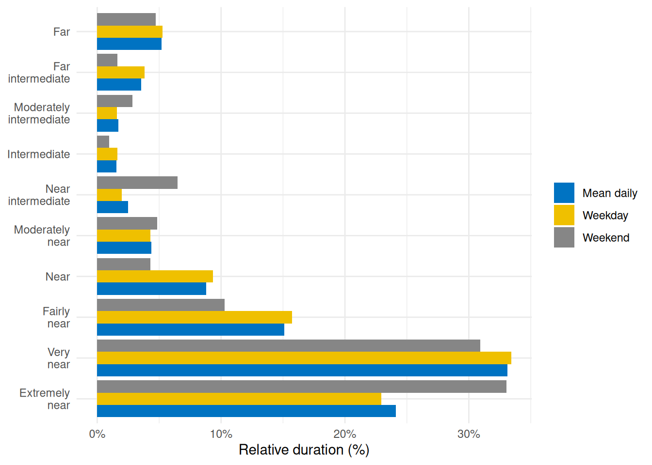
##### Duration within distance ranges
First, we define a set of distance breakpoints and descriptive labels for each range. Depending on the type of device (valid measurement range) and theoretical assumptions, these could be chosen differently by the user:
```{r}
#| filename: Defining distance ranges (in cm)
dist_breaks <- c(15, 20, 30, 40, 50, 60, 70, 80, 90, 100, Inf)
dist_labels <- c(
    "Extremely near",          # [15, 20)
    "Very near",               # [20, 30)
    "Fairly near",             # [30, 40)
    "Near",                    # [40, 50)
    "Moderately near",         # [50, 60)
    "Near intermediate",       # [60, 70)
    "Intermediate",            # [70, 80)
    "Moderately intermediate", # [80, 90)
    "Far intermediate",        # [90, 100)
    "Far"                      # [100, Inf)
  )
```
Now we cut the distance data into these ranges and compute the daily duration spent in each range. As we set values above 120 cm to `NA` in the preprocessing stage (see [Supplement](supplement.qmd)), these would be missing from this analysis. However, we know that a value of, e.g., 180cm, while not accurate to within a few centimeters, is almost certainly greater than 100cm. Thus, we will create a column that sets these values to 120cm. As long as only duration, and not average distance is required, this remains valid.
```{r}
#| filename: Recode distance values > 120cm
dataCC <-
  dataCC |>
  mutate(Dis_cap = replace_when(Dis,
                                Dis_status == "over 120cm" ~ 120))
```
```{r}
#| label: tbl-ranges
#| filename: Calculate daily duration within viewing distance range
#| tbl-cap: "Daily duration in each viewing distance range"
dataCC |>
mutate(Dis_range = cut(Dis_cap, breaks = dist_breaks, labels = dist_labels)) |> #<1>
drop_na(Dis_range) |> #<2>
group_by(Dis_range, .add = TRUE) |> # <3>
durations(Dis_cap) |> # <4>
pivot_wider(names_from = Dis_range, values_from = duration) |> # <5>
ungroup() |>
mean_daily(prefix = "") |>
pivot_longer(-Date) |>
pivot_wider(names_from = Date) |>
mutate(name = factor(name, levels = rev(dist_labels))) |>
arrange(name) |>
gt() |>
fmt_duration(input_units = "seconds", output_units = "minutes") # <6>
```
1. Categorize distances
2. Remove intervals with no data
3. Group by distance range (in addition to the date)
4. Duration per range per day
5. Pivot data from long to wide format (ranges as columns)
6. Convert seconds to minutes
To visualize this, @fig-ranges illustrates the relative proportion of time spent in each distance range:
```{r}
#| label: fig-ranges
#| filename: Plot time spent within each viewing distance range
#| fig-cap: "Percentage of total time spent in each viewing distance range for an average day (mean daily), average weekday, or weekend"
dataCC |>
mutate(Dis_range = cut(Dis_cap, breaks = dist_breaks, labels = dist_labels)) |> #<1>
drop_na(Dis_range) |> #<1>
group_by(Dis_range, .add = TRUE) |> #<1>
durations(Dis_cap) |> #<1>
group_by(Dis_range) |> #<1>
mean_daily(prefix = "") |> #<1>
ungroup() |> #<1>
mutate(Dis_range = forcats::fct_relabel(Dis_range, \(x) str_replace(x, " ", "\n"))) |>
mutate(duration = duration/sum(duration), .by = Date) |> #<2>
ggplot(aes(x = Dis_range, y = duration, fill = Date)) +
geom_col(position = "dodge") +
scale_y_continuous(labels = scales::label_percent()) +
ggsci::scale_fill_jco() +
theme_minimal() +
labs(y = "Relative duration (%)", x = NULL, fill = NULL) +
coord_flip()
ggsave("manuscript/figures/Figure3.pdf",
device = cairo_pdf,
width = 7,
height = 5)
```
1. Broadly, this portion repeats the prior code cell
2. Convert to percentage of daily total
:::
#### Frequency of continuous near work
Continuous near-work can be understood as sustained viewing within a near distance for some minimum duration, allowing only brief interruptions. We use LightLogR’s `cluster` function to identify episodes of continuous near work. Here, we define a near-work episode as viewing distance between 20 cm and 60 cm that lasts at least 15 minutes, with interruptions of up to 30 seconds allowed (meaning short breaks ≤30 secs do not end the episode). Using [extract_clusters()](https://tscnlab.github.io/LightLogR/reference/extract_clusters.html) with those parameters, we count how many such episodes occur per day. It should be noted that the adjustment of these parameters is not only possible, but should actively be done by researchers to gauge meaningful insights into the data at hand. If, for example, a participant is predominantly indoors, e.g., at work at a desk, a higher time threshold, like 30 minutes, might not meaningfully change the outcome, as the episodes last longer anyways. For mixed or outdoor situations, however, 30 minutes might be too long, and not catch shorter but still meaningful episodes, which was the case here.
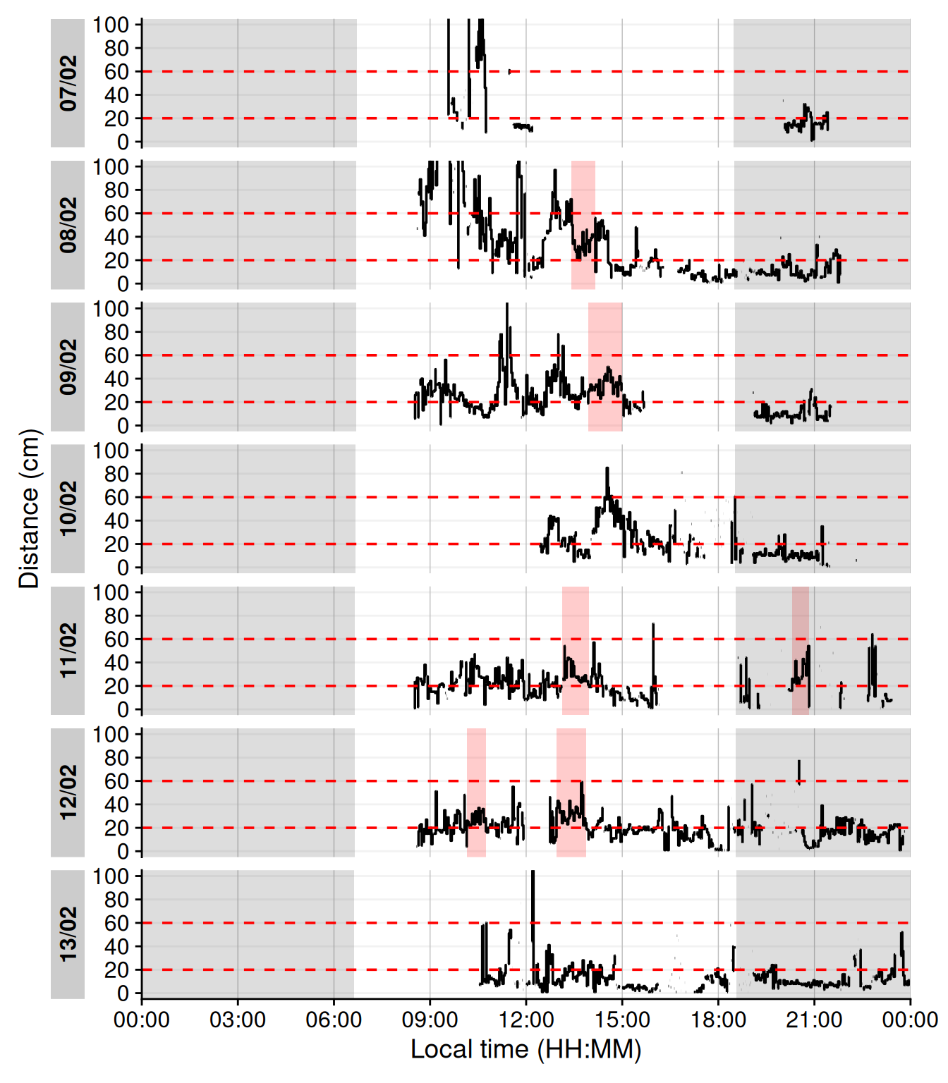
@tbl-continuousnear summarizes the average frequency of continuous near-work episodes per day, and @fig-visbreak provides an example visualization of these episodes on the distance time series.
```{r}
#| label: tbl-continuousnear
#| filename: Calculate the frequency of continuous near-work episodes per day
#| tbl-cap: "Frequency of continuous near-work episodes per day"
dataCC |>
extract_clusters(
Dis >= 20 & Dis < 60, # <1>
cluster.duration = "15 mins", # <2>
interruption.duration = "30 secs", # <3>
drop.empty.groups = FALSE # <4>
) |>
summarize_numeric(remove = c("start", "end", "epoch", "duration"), # <5>
add.total.duration = FALSE) |> # <5>
mean_daily(prefix = "Frequency of near-work ") |> # <6>
gt() |> fmt_number()
```
1. Condition: near-work distance
2. Minimum duration of a continuous episode
3. Maximum gap allowed within an episode
4. Keep days with zero episodes in output
5. Count number of episodes per day
6. Compute daily mean frequency
```{r}
#| label: fig-visbreak
#| filename: Plot continuous near-work episodes
#| fig-cap: "Example of continuous near-work episodes. Red shaded areas indicate periods of continuous near work (20–60 cm for ≥15 min, allowing ≤30 secs interruptions). Black trace is viewing distance over time; red dashed lines mark the 20 cm and 60 cm boundaries. Grey shaded areas indicate nighttime."
#| warning: false
#| fig-height: 8
dataCC |> # <1>
add_clusters(# <1>
Dis >= 20 & Dis < 60,# <1>
cluster.duration = "15 mins",# <1>
interruption.duration = "30 secs"# <1>
) |> # <1>
gg_day(y.axis = Dis, y.axis.label = "Distance (cm)", geom = "ribbon",
fill = "gold", alpha = 0.2, col = "black", linewidth = 0.3,
format.day = "%a", #<2>
y.scale = "identity", y.axis.breaks = seq(0,100, by = 20)) |>
gg_photoperiod(coordinates) |># <3>
gg_states(state, fill = "red", alpha = 0.75) + # <4>
geom_hline(yintercept = c(20, 60), col = "red", linetype = "dashed") +
coord_cartesian(ylim = c(0,100)) +
theme(legend.position = "bottom")
```
1. As in code cell above
2. Label weekdays instead of dates
3. Add photoperiod information
4. Add state bands
```{r}
#| echo: false
#| output: false
ggsave("manuscript/figures/Figure4.pdf",
device = cairo_pdf,
width = 9,
height = 9)
```
#### Near-work episodes
Beyond frequency, we can characterize near-work episodes by their duration and typical viewing distance. This section extracts all near-work episodes (using a 5-second minimum duration to capture more routine near-work bouts) and summarizes three aspects:
1. frequency (count of episodes per day),
2. average duration of episodes, and
3. average distance during those episodes.
These results are combined in @tbl-nearworkepisodes.
```{r}
#| label: tbl-nearworkepisodes
#| filename: Calculate near-work episodes
#| tbl-cap: "Near-work episodes: mean duration, mean viewing distance, and frequency"
dataCC |>
extract_clusters(
Dis >= 20 & Dis < 60,
cluster.duration = "5 secs", # <1>
interruption.duration = "20 secs",
drop.empty.groups = FALSE
) |>
extract_metric(dataCC, distance = mean(Dis, na.rm = TRUE)) |> # <2>
summarize_numeric(remove = c("start", "end", "epoch"), # <3>
prefix = "", #<3>
add.total.duration = FALSE) |> #<3>
mean_daily(prefix = "") |> # <4>
gt() |> # <5>
fmt_number(c(distance, episodes), decimals = 0) |> # <5>
cols_units(distance = "cm") # <5>
```
1. Minimal duration to count as an episode (set to interval level of `dataCC`)
2. Calculate mean distance during each episode
3. Calculate averages for all numeric columns per group
4. Daily averages for each metric
5. Table generation
> In the code cell above, `extract_metric(..., distance = mean(Dis, ...))` computes the mean viewing distance during each episode, and the subsequent `summarize_numeric` and `mean_daily` steps derive daily averages of episode count, duration, and distance.
#### Visual breaks
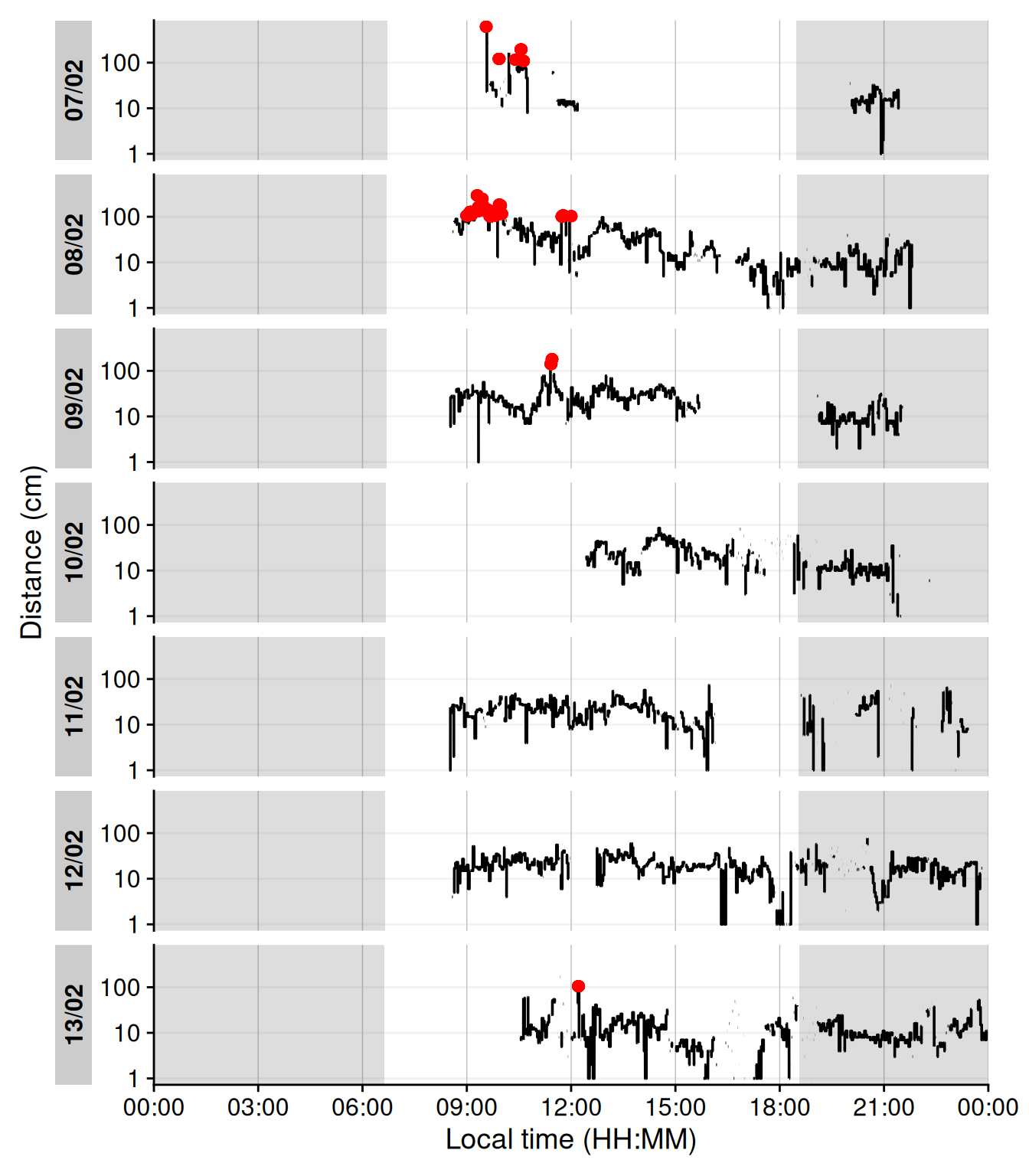
`Visual breaks` as defined in this article, require a minimum break-length, and the previous episode is important. This leads to a two step process, where we first extract instances of `Distance` above 100 cm, before we filter for a (valid) previous duration of at maximum 20 minutes. @tbl-visualbreaks provides the daily frequency of visual breaks and @fig-cluster shows when these occur. While visual breaks are not a commonly used metric, they highlight the powerful detection mechanisms that are available.
```{r}
#| label: tbl-visualbreaks
#| filename: Calculate visual breaks
#| tbl-cap: "Frequency of visual breaks"
dataCC |>
extract_states(State.colname = vis.break, # <1>
State.expression = Dis >= 100, # <1>
drop.empty.groups = FALSE, # <1>
group.by.state = FALSE) |> # <1>
arrange(start, .by_group = TRUE) |> #<2>
filter(!is.na(lag(vis.break)), #<3>
lag(duration) <= duration("20 mins"), #<4>
vis.break) |> #<5>
summarize_numeric(remove = c("start", "end", "epoch", "is.cluster", "duration"), #<6>
prefix = "", #<6>
add.total.duration = FALSE) |> #<6>
mean_daily(prefix = "Daily ") |> # <7>
gt() |> #<8>
fmt_number(decimals = 1) #<8>
```
1. Define the condition, greater 100 cm away, and store it in a variable `vis.break`. Empty groups (days), should not be dropped, and the new state should not be a new grouping variable.
2. Because `extract_states()` sorts the output by the new states, we need to arrange them in timely order
3. Only keep instances where the previous condition is not `NA` (i.e., we do not know whether it is below or above 100 cm distance)
4. Only keep instances, where the previous conditions is at max 20 minutes
5. Only keep instances, where the current condition is equal to or greater 100 cm distance
6. Count the number of episodes
7. Calculate daily means
8. Table generation
```{r}
#| label: fig-cluster
#| filename: Plot visual breaks
#| fig-cap: "Plot of visual breaks (red vertical bars). Black traces show distance measurement data. Grey shaded areas show nighttime between civil dusk and civil dawn"
#| warning: false
#| fig-height: 8
dataCC |> # <1>
add_states( # <1>
dataCC |> # <2>
extract_states(State.colname = vis.break, # <2>
State.expression = Dis >= 100, # <2>
drop.empty.groups = FALSE, # <2>
group.by.state = FALSE) |> # <2>
arrange(start) |> # <2>
filter(!is.na(lag(vis.break)), # <2>
lag(duration) <= duration("20 mins"), # <2>
vis.break) # <2>
)|> # <1>
gg_day(y.axis = Dis, y.axis.label = "Distance (cm)", geom = "ribbon",
linewidth = 0.3, col = "black", y.axis.breaks = seq(0,100, by = 20),
alpha = 0.25, fill = "gold", y.scale = "identity", format.day = "%a") |>
gg_photoperiod(coordinates) |> # <3>
gg_states(vis.break, fill = "red", alpha = 1) + # <4>
geom_hline(yintercept = 100, linetype = "dashed") +
coord_cartesian(xlim = c(6,18)*60*60)
```
1. Add the states to the data
2. As in the code cell above
3. Add photoperiod information to the plot
4. Highlight the points
```{r}
#| echo: false
#| output: false
ggsave("manuscript/figures/Figure5.pdf",
device = cairo_pdf,
width = 9,
height = 9)
```
#### Distance with spatial distribution
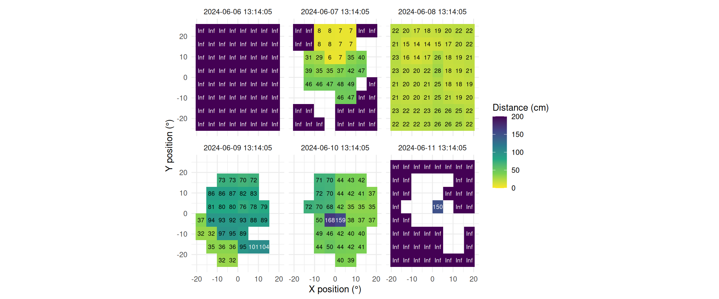
The `Clouclip` device outputs a singular measure for distance, while the visual environment in natural conditions contains many distances, depending on the solid angle and direction of the measurement. A device like the `VEET` increases the spatial resolution of these measurements, allowing for more in-depth analyses of the size and position of an object within the field of view. In the case of the `VEET`, data are collected from an 8x8 measurement grid, spanning 52° vertically and 41° horizontally. @fig-VEET-distance shows sample observations from six different days at the same time.
```{r}
#| filename: Collect plot partials to plot the spatial distance grids
extras <- list(
  geom_tile(),
  scale_fill_viridis_c(direction = -1, limits = c(0, 200),
                       oob = scales::oob_squish_any),
  scale_color_manual(values = c("black", "white")),
  theme_minimal(),
  guides(colour = "none"),
  geom_text(aes(label = (dist1/10) |> round(0), colour = dist1>1000), size = 2.5),
  coord_fixed(),
  labs(x = "X position (°)", y = "Y position (°)",
       fill = "Distance (cm)", alpha = "Confidence (0-255)"))
```
```{r}
#| label: fig-VEET-distance
#| filename: Plot spatial distance grids for different days
#| fig-cap: "Example observations of the measurement grid at 1:14 p.m. for each measurement day. Text values show distance in cm. Empty grid points show values with low confidence. Zero-distance values were replaced with infinite distance and plotted despite low confidence."
#| fig-height: 5
#| message: false
#| warning: false
#| fig-width: 12
dataVEET3 |>
filter_Time(start = "13:14:02", length = "00:00:05") |> #<1>
mutate(dist1 = ifelse(dist1 == 0, Inf, dist1)) |> #<2>
filter(conf1 >= 0.1 | dist1 == Inf) |> #<3>
ggplot(aes(x=x.pos, y=y.pos, fill = dist1/10))+ #<4>
extras + #<4>
facet_wrap(~Datetime) #<5>
```
1. Choose a particular observation
2. Replace 0 distances with infinity
3. Remove data that has less than 10% confidence
4. Plot the data and add the plot partials from the code cell above
5. Show one plot per day
```{r}
#| echo: false
#| output: false
ggsave("manuscript/figures/Figure6.pdf",
device = cairo_pdf,
width = 8,
height = 6)
```
This spatial resolution necessitates a change in the data format. When we try to apply the preprocessed `VEET` data to the functions described above for the `Clouclip` device, we run into issues. This is because each time point is repeated 64 times to include the 64 different spatial positions. `LightLogR` expects unique time points for all observations within each group (in our case days within participants). To use these distance data in the framework shown above for the `Clouclip` device, a sensible method to condense the data has to be applied. There are many ways how a spatially resolved distance measure could be utilized for analysis:
- Where in the field of view are objects in close range?
- How large are near objects in the field of view?
- How varied are distances within the field of view?
- How close are objects / is viewing distance in a region of interest within the field of view?
Possible methods include:
- average across all (high confidence) distance values within the grid
- closest (high confidence) distance within the grid
- (high confidence) values at or around a given grid position, e.g., ±10 degrees around the central view (0°)
Many more options are available based on the spatial dataset, e.g., condensation rules based on the number of points in the grid with a given condition, or the variation within the grid.
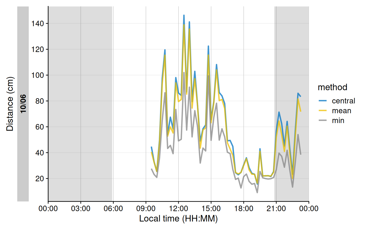
We will demonstrate these three methods for a single day (`2024-06-10`), all leading to a data structure akin to the `Clouclip`, i.e., to be used for further calculation of visual experience metrics.
```{r}
#| label: fig-VEET-distance_methods
#| filename: Calculating and plotting method results
#| fig-cap: "Comparison of condensation methods for spatial grid of distance measurements. The lines represent an average across all data points (yellow), the minimum distance (grey), or the central 10° (blue). Data points with confidence less than 10% were removed prior to calculation."
#| fig-height: 5
#| fig-width: 8
dataVEET3_part <- #<1>
dataVEET3 |> #<1>
filter_Date(start = "2024-06-10", length = "1 day") #<1>
dataVEET3_condensed <-
dataVEET3_part |>
group_by(Datetime, .add = TRUE) |> #<2>
filter(conf1 >= 0.1) |> #<3>
summarize(
distance_mean = mean(dist1), #<4>
distance_min = min(dist1), #<5>
distance_central = mean(dist1[between(x.pos, -10,10) & between(y.pos, -10,10)]), #<6>
n = n(), #<7>
.groups = "drop_last"
)
dataVEET3_condensed |>
aggregate_Datetime("15 mins", numeric.handler = \(x) mean(x, na.rm = TRUE)) |> #<8>
remove_partial_data(by.date = TRUE) |> #<9>
pivot_longer(contains("distance"), #<10>
names_to = c(".value", "method"), #<10>
names_pattern = "(distance)_(mean|min|max|central)" #<10>
) |> #<10>
gg_day(y.axis = distance/10, #<11>
geom = "line", #<11>
aes_col = method,#<11>
group = method,#<11>
linewidth = 1, #<11>
alpha = 0.75, #<11>
y.scale = "identity",#<11>
y.axis.breaks = seq(0,150, by = 20), #<11>
y.axis.label = "Distance (cm)"#<11>
) |> #<11>
gg_photoperiod(coordinates) #<11>
```
1. Filter one day
2. Group additionally by every observation
3. Remove data with low confidence
4. Average across all distance values
5. Closest across all distance values
6. Central distance
7. Number of (valid) grid points
8. Aggregate to 15 minute data
9. Remove data points that fall exactly on midnight of the following day
10. Pivoting the method results from wide to long for plotting
11. Setting up the plot for distance.
```{r}
#| echo: false
#| output: false
ggsave("manuscript/figures/Figure7.pdf",
device = cairo_pdf,
width = 7,
height = 4)
```
As can be seen in @fig-VEET-distance_methods, while the overall pattern is similar regardless of the used method, there are notable differences between the methods, which will consequently affect downstream analyses. Most importantly, the process of condensation has to be well documented and reproducible, as shown above. Any of these data could now be used to calculate the `frequency of continuous near work`, `visual breaks`, or `near-work episodes` as described above.
### Light {#light}
To illustrate light exposure metrics, we turn to a different dataset, this one taken from the `VEET` device’s illuminance data, which capture a broader range of lighting conditions (though both device types are able to capture broadly the same range of illuminance). We import the `VEET` ambient light data (already preprocessed to have regular 5-second intervals as described above) and briefly examine its distribution.
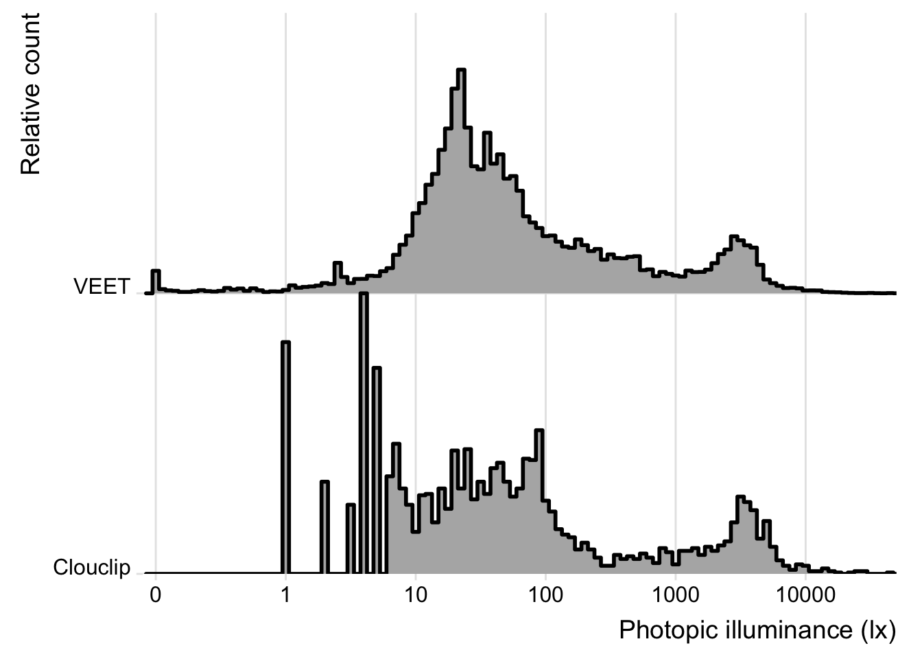
**Illuminance distribution**: The `VEET` data include indoor and outdoor exposures up to several thousand lux. The contrast between the two settings is evident from comparing histograms of the two datasets’ lux values (`Clouclip` and `VEET`), where the main peak is similarly positioned between 10 and 100 lx, but the tails differ. The `VEET` illuminance histogram (see @fig-hist) shows a heavily skewed distribution with a considerable number of zero lx values (indicating intervals of complete darkness or the sensor being covered) and a long tail extending to very high lux values. Such zero-inflated and skewed data are common in wearable light measurements [@ZaunerEtAl2025JBR]. The `Clouclip`, however, shows a minimal value of 1 lx, and worse discrimination below 10 lx (see @fig-hist). Additionally, the `Clouclip` was not recording when the device was not worn, e.g., during sleep (`sleep mode`), compared to the continuous recording of `VEET` devices, where non-wear data was removed in the preprocessing (see [Supplement](supplement.qmd)), based on the activity sensors of the device.
```{r}
#| label: fig-hist
#| column: margin
#| warning: false
#| echo: false
#| fig-cap: "Histogram of illuminance values from the VEET and Clouclip dataset (5-second data). Indoor light exposure mainly occurs arount 10^1 to 10^2 lx. Outdoor (day)light exposures in bright conditions are mostly around 10^3 to 10^4 lx."
dataCC |>
bind_rows(dataVEET) |>
ggplot(aes(x = Lux)) +
labs(x = "Photopic illuminance (lx)", y = "Relative count") +
ggridges::geom_density_ridges(binwidth = 0.05, aes(y = Id), linewidth = 1,
stat = "binline", scale = 1) +
ggridges::theme_ridges() +
guides(fill = "none")+
scale_x_continuous(trans = "symlog", breaks = c(0, 1, 10, 100, 1000, 10000),
) +
coord_cartesian(xlim = c(-0.1, 5*10^4), ylim = c(1, 3), expand = FALSE)
ggsave("manuscript/figures/Figure8.pdf",
device = cairo_pdf,
width = 7,
height = 5)
```
After confirming that the `VEET` data cover a broad dynamic range of lighting, we proceed with calculating light exposure metrics. (The VEET data had been cleaned for gaps and irregularities as described earlier, and non-wear times were removed; see [Supplement 1](supplement.qmd) for the details.)
#### Average light exposure {#sec-avelight}
A basic metric is the average illuminance over the day. @tbl-lightexposure shows the mean illuminance (in lux) for weekdays, weekends, and the overall daily mean, calculated directly from the raw lux values.
```{r}
#| label: tbl-lightexposure
#| filename: Calculating mean light exposure per day
#| tbl-cap: "Mean light exposure (illuminance) per day"
dataVEET |>
  select(Id, Date, Datetime, Lux) |>
  summarize_numeric(prefix = "mean ", remove = c("Datetime")) |>
  to_mean_daily() |>
  fmt_number(decimals = 1) |>
  cols_hide(`average episodes`) |>
  cols_label(`average mean Lux` = "Mean photopic illuminance (lx)")
```
However, because illuminance data tend to be extremely skewed and contain many zero values (periods of darkness), the arithmetic mean can be [misleading](https://tscnlab.github.io/LightLogR/articles/log.html). A common approach is to apply a logarithmic transform to illuminance before averaging, which down-weights extreme values and accounts for the multiplicative nature of light intensity effects. LightLogR provides helper functions [`log_zero_inflated()`]((https://tscnlab.github.io/LightLogR/reference/log_zero_inflated.html)) and its inverse [`exp_zero_inflated()`](https://tscnlab.github.io/LightLogR/reference/log_zero_inflated.html) to handle log-transformation when zeros are present (by adding a small offset before log, and back-transforming after averaging). Using this approach, we recompute the daily mean illuminance. The results in @tbl-lightexposure2 show that the log-transformed mean (back-transformed to lux) is much lower, reflecting the fact that for much of the time illuminance was near zero. This transformed mean is often more representative of typical exposure for skewed data.
```{r}
#| label: tbl-lightexposure2
#| filename: Calculating mean light exposure per day with log transformation
#| tbl-cap: "Mean light exposure per day (after logarithmic transformation to account for zero inflation and skewness)"
dataVEET |>
select(Id, Date, Datetime, Lux) |>
mutate(Lux = Lux |> log_zero_inflated()) |> # <1>
summarize_numeric(prefix = "mean ", remove = c("Datetime")) |>
mean_daily(prefix = "") |> # <2>
mutate(`mean Lux` = `mean Lux` |> exp_zero_inflated()) |> # <3>
gt() |> fmt_number(decimals = 1) |> cols_hide(episodes) |>
cols_label(`mean Lux` = "Mean photopic illuminance (lx)")
```
1. Log transform with zero handling (base 10)
2. Calculate daily mean of log-lux
3. Back-transform to lux
#### Duration in high-light (outdoor) conditions {#sec-outdoorlight}
Another important metric is the amount of time spent under bright light, often used as a proxy for outdoor exposure. We define thresholds corresponding to outdoor light levels (e.g. 1000 lx and above). Here, we categorize each 5-second interval of illuminance into bands: Outdoor bright (≥1000 lx), Outdoor very bright (≥2000 lx), and Outdoor extremely bright (≥3000 lx). We then sum the duration in each category per day.
While daylight levels can far exceed the recorded light levels, those are usually recorded with direct sunlight and without obstruction. Under normal viewing conditions, at eye level, and avoiding glare, daylight levels of a few thousand lux are at the higher end of the distribution [@murukesu2025ADID]. @fig-hist shows a bimodal distribution, with the right mode representing outdoor lighting conditions. In a 2023 review of light dosimeters to investigate the light-myopia relationship [@Honekopp2023ClinOphthalmol], 1000 lx was the predominant cutoff value to distinguish indoor vs. outdoor environments. It is not, however, without critique, and both other thresholds [@pattersongentile2025] and classification methods are proposed [@tabandeh2025].
```{r}
#| filename: Define outdoor illuminance thresholds (in lux)
out_breaks <- c(0, 1e3, 2e3, 3e3, Inf)
out_labels <- c(
    "Indoor",                  # [0, 1000) lx
    "Outdoor bright",          # [1000, 2000) lx
    "Outdoor very bright",     # [2000, 3000) lx
    "Outdoor extremely bright" # [3000, ∞) lx
  )

dataVEET <- dataVEET |>
  mutate(Lux_range = cut(Lux, breaks = out_breaks, labels = out_labels))
```
Now we compute the mean daily duration spent in each of these outdoor light ranges (@tbl-outdoor):
```{r}
#| label: tbl-outdoor
#| filename: Calculate the mean daily duration spent in each light range
#| tbl-cap: "Average daily duration in outdoor-equivalent light conditions"
dataVEET |>
  drop_na(Lux_range) |>
  group_by(Lux_range, .add = TRUE) |>
  durations(Lux) |>
  pivot_wider(names_from = Lux_range, values_from = duration) |>
  to_mean_daily("") |>
  fmt_duration(input_units = "seconds", output_units = "minutes")
```
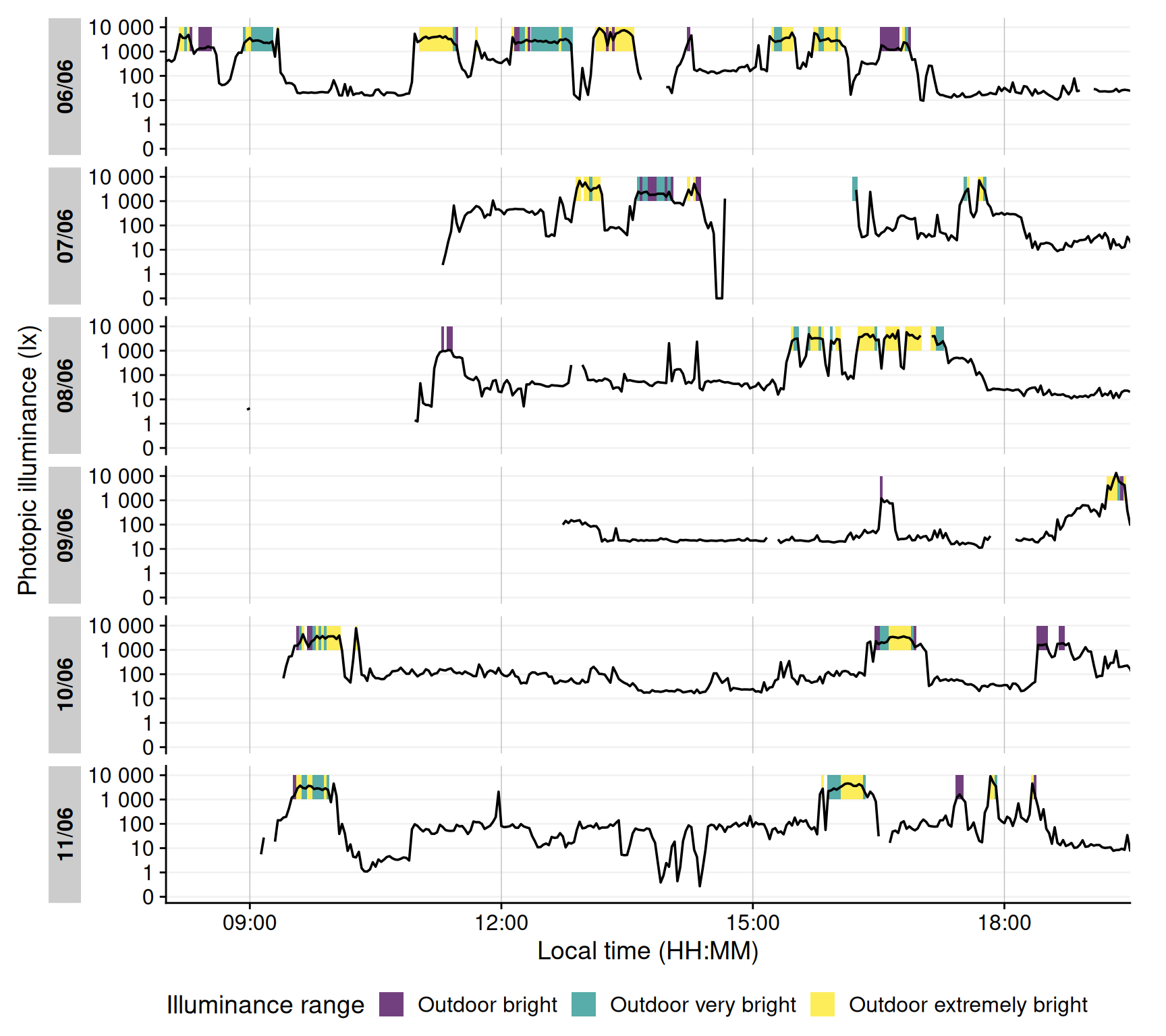
It is also informative to visualize when these high-light conditions occurred. @fig-outdoor shows a timeline plot with periods of outdoor-level illuminance highlighted in color. In this example, violet denotes ≥1000 lx, green ≥2000 lx, and yellow ≥3000 lx. Grey shading indicates nighttime (from civil dusk to dawn) for context.
```{r}
#| fig-height: 8
#| fig-width: 9
#| warning: false
#| filename: Visualize time spent outdoors
#| label: fig-outdoor
#| fig-cap: "Outdoor light exposure over time with 2-minute interval. Colored bands indicate periods when illuminance exceeded outdoor thresholds for at least half of each interval: violet for ≥1000 lx, green for ≥2000 lx, and yellow for ≥3000 lx. Grey shaded regions denote night (from civil dusk to dawn)."
dataVEET |>
aggregate_Datetime("2 mins", type = "floor") |> #<1>
mutate(Lux_range = fct_recode(Lux_range, NULL = "Indoor")) |> #<2>
gg_day(y.axis = Lux, #<3>
y.axis.label = "Photopic illuminance (lx)", #<3>
geom = "line", #<3>
jco_color = FALSE) |> #<3>
gg_states(Lux_range, aes_fill = fct_rev(Lux_range), #<4>
alpha = 0.75, ymin = 10^3, ymax = 10^4) + #<4>
scale_fill_viridis_d() +
labs(fill = "Illuminance range") +
theme(legend.position = "bottom") +
coord_cartesian(xlim = c(8, 19.5)*3600) #<5>
```
1. Aggregating data to 5-minute bins
2. Removing the indoor condition
3. Setting up the basic plot
4. Adding state information on the illuminance ranges
5. Setting the x-axis limits to cover daytime hours
```{r}
#| echo: false
#| output: false
ggsave("manuscript/figures/Figure9.pdf",
device = cairo_pdf,
width = 9,
height = 7)
```
#### Frequency of transitions from indoor to outdoor light
We next consider how often the subject moved from an indoor light environment to an outdoor-equivalent environment. We operationally define an "outdoor transition" as a change from \<1000 lx to ≥1000 lx. Using the cleaned `VEET` data, we extract all instances where illuminance crosses that threshold from below to above.
@tbl-changesoutdoor shows the average number of such transitions per day. Note that if data are recorded at a fine temporal resolution (5 s here), very brief excursions above 1000 lx could count as transitions and inflate this number. Indeed, the initial count is fairly high, reflecting fleeting spikes above 1000 lx that might not represent meaningful outdoor exposures.
```{r}
#| label: tbl-changesoutdoor
#| filename: Calculate the number of transitions from indoor to outdoor
#| tbl-cap: "Average daily count of transitions from indoor (<1000 lx) to outdoor (≥1000 lx) lighting when looking at 5-second epochs"
dataVEET |>
extract_states(Outdoor, Lux >= 1000, group.by.state = FALSE) |> # <1>
filter(!lead(Outdoor) & Outdoor) |> #<2>
summarize_numeric(prefix = "mean ",
remove = c("Datetime", "Outdoor", "start", "end", "duration"),
add.total.duration = FALSE) |>
mean_daily(prefix = "") |>
gt() |>
fmt_number(episodes, decimals = 0) |>
fmt_duration(`mean epoch`, input_units = "seconds", output_units = "seconds")
```
1. Label each interval as Outdoor (Lux≥1000) or not
2. Find instances where the previous interval was "indoor" and current is "outdoor"
To obtain a more meaningful measure, we can require that the outdoor state persists for some minimum duration to count as a true transition (filtering out momentary fluctuations around the 1000 lx mark). For example, we can require that once ≥1000 lx is reached, it continues for at least 5 minutes (allowing short interruptions up to 20 s). @tbl-changesoutdoor2 applies this criterion, resulting in a lower, more plausible transition count.
```{r}
#| label: tbl-changesoutdoor2
#| filename: Calculate the number of transitions from indoor to outdoor with clusters
#| tbl-cap: "Daily indoor-to-outdoor transition count (requiring ≥5 min duration of ≥1000 lx to count)"
dataVEET |>
  extract_clusters(Lux >= 1000,
                   cluster.duration = "5 min",
                   interruption.duration = "20 secs",
                   return.only.clusters = FALSE,
                   drop.empty.groups = FALSE) |>
  filter(!lead(is.cluster) & is.cluster) |>
  summarize_numeric(prefix = "mean ",
    remove = c("Datetime", "start", "end", "duration"),
    add.total.duration = FALSE) |>
  mean_daily(prefix = "") |>
  gt() |> fmt_number(episodes, decimals = 0)
```
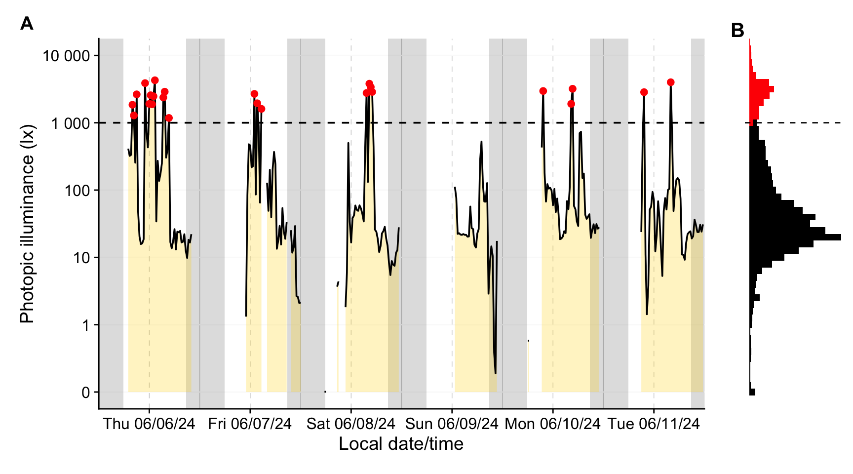
Another possibility would be to check for stronger changes between consecutive episodes, or aggregate the data further for average values across longer time spans (see @fig-aggregate).
```{r}
#| filename: Aggregate time series to coarser intervals
plot_timeline <-
dataVEET |>
ungroup() |>
aggregate_Datetime( #<1>
"20 minutes", #<2>
type = "floor",#<3>
numeric.handler = \(x) median(x, na.rm = TRUE)) |> #<4>
gg_days(y.axis = Lux, geom = "ribbon", facetting = FALSE,
y.axis.label = "Photopic illuminance (lx)",
fill = "gold", alpha = 0.25, col = "black") |>
gg_photoperiod(coordinates) +
geom_hline(yintercept = 1000, linetype = "dashed") +
geom_point(data = \(x) filter(x, Lux > 1000), col = "red") +
coord_cartesian(ylim = c(0, 10^4))
```
1. Function to reduce the interval through aggregation.
2. Bins of arbitrary length are created (here `20 minutes`)
3. Values are sorted into these bins (`type = "floor"` specifies that values are always sorted in the next lower bin)
4. The function provides sensible default handlers for data types like numeric, text, factor, boolean, etc.. For numeric, the default is `mean` and `NA`s propagate. Here, we set the `median` as handler and ignore missing values.
```{r}
#| fig-height: 5
#| fig-width: 9
#| warning: false
#| filename: Plot aggregated dataset
#| label: fig-aggregate
#| fig-cap: "A: Outdoor light exposure over time with 20-minute interval. Grey shaded regions denote night (from civil dusk to dawn). Red points denote intervals with a median illuminance above 1000 lx. B: Histogram of 5-second data (color as panel A)"
plot_histogram <-
dataVEET |>
ggplot(aes(y=Lux)) +
geom_histogram(binwidth = 0.1, aes(fill = Lux > 1000)) +
scale_y_continuous(trans = "symlog") +
guides(fill = "none") +
scale_fill_manual(values = c("black", "red")) +
geom_hline(yintercept = 1000, linetype = "dashed") +
coord_cartesian(ylim = c(0, 10^4)) +
theme_void()
plot_timeline + plot_histogram + #<1>
plot_layout(widths = c(6, 1)) + #<1>
plot_annotation(tag_levels = "A") + #<1>
theme(plot.tag = element_text(size = 15, face = "bold")) #<1>
```
1. Plot composition using the {patchwork} package
```{r}
#| echo: false
#| output: false
ggsave("manuscript/figures/Figure10.pdf",
device = cairo_pdf,
width = 9,
height = 5)
```
#### Longest sustained bright-light period
The final light exposure metric we illustrate is the longest continuous period above a certain illuminance threshold (often termed longest period above threshold, e.g. PAT<sub>1000</sub> for 1000 lx). This gives us a sense of the longest outdoor exposure in a day. Along with it, one might report the total duration above that threshold in the day (TAT<sub>1000</sub>). While we could derive these from the earlier analyses, LightLogR provides dedicated [metric](https://tscnlab.github.io/LightLogR/articles/Metrics.html) functions for such calculations, which can compute multiple related metrics at once.
Using the function [period_above_threshold()](https://tscnlab.github.io/LightLogR/reference/period_above_threshold.html) for PAT and [duration_above_threshold()](https://tscnlab.github.io/LightLogR/reference/duration_above_threshold.html) for TAT, we calculate both metrics for the 1000 lx threshold. @tbl-periodoutdoor shows the mean of these metrics across days (i.e., average longest bright period and average total bright time per day).
```{r}
#| label: tbl-periodoutdoor
#| filename: Calculate PAT1000 and TAT1000
#| tbl-cap: "Longest period and total duration illuminance above 1000 lx (PAT1000 and TAT1000)"
dataVEET |>
  summarize(
    period_above_threshold(
      Lux, Datetime, threshold = 1000, na.rm = TRUE, as.df = TRUE),
    duration_above_threshold(
      Lux, Datetime, threshold = 1000, na.rm = TRUE, as.df = TRUE),
    .groups = "keep"
  ) |>
  rename_with(\(x) str_replace(x, "1000", "1000 lx")) |>
  to_mean_daily("")
```
#### Merging data streams
Note that while imports from different devices can be [merged](https://tscnlab.github.io/LightLogR/reference/join_datasets.html), devices differ in their sensors, electronics, housing or diffuser form factors, and on-device data-processing pipelines. All of these factors affect the comparability of measurements, even when devices output the same variable (e.g., illuminance or distance). If data from different devices with the same measurement variable are to be merged, the corresponding variable names should be standardized beforehand - for example, renaming `Lux` and `LIGHT` to `illuminance`. If we wanted to analyse the `VEET` data together with the `Clouclip` data, for example, we would not have to rename anything, as both carry their illuminance measurements in the variable `Lux`. The following example shows how the combination of datasets would lead to a combined dataset, and how that would affect analysis outcomes. **It is the responsibility of the researcher to perform device calibration and/or checks for a similar measurement fidelity.**
```{r}
#| filename: Merge Clouclip and VEET data
#| label: tbl-merge
#| tbl-cap: "Overview of the merged dataset"
data <- join_datasets(dataCC, dataVEET)
data |> summary_overview(Lux, threshold.missing = 0.5) |> gt() |> sub_missing()
```
We will reuse the example from @sec-avelight, but instead of one participant, we now have data from two devices and participants
```{r}
#| label: tbl-relight
#| tbl-cap: "Recalculation of the mean light exposure per day (after logarithmic transformation to account for zero inflation and skewness) with the merged dataset"
#| filename: Re-calculate mean photopic illuminance with the merged dataset
data |> # <1>
select(Id, Date, Datetime, Lux) |> # <2>
mutate(Lux = Lux |> log_zero_inflated()) |> # <2>
summarize_numeric(prefix = "mean ", remove = c("Datetime")) |> # <2>
mean_daily(prefix = "") |> # <2>
mutate(`mean Lux` = `mean Lux` |> exp_zero_inflated()) |> # <2>
gt() |> fmt_number(decimals = 1) |> cols_hide(episodes) |> # <2>
cols_label(`mean Lux` = "Mean photopic illuminance (lx)")# <2>
```
1. Instead of `dataVEET` we now supply the merged `data` object
2. Verbatim from @sec-avelight
### Spectrum
The `VEET` device’s spectral sensor provides multimodal data beyond simple lux values, but it requires reconstruction of the actual light spectrum from raw sensor counts. We processed the spectral sensor data in order to compute two example spectrum-based metrics. Detailed data import, normalization, and spectral reconstruction steps are given in [Supplement 1](supplement.qmd); here we present the resulting metrics. Briefly, the `VEET`’s spectral sensor recorded counts in nine wavelength bands (roughly 415 nm to 910 nm), plus a `Dark`, a `Clear`, and a flicker detection channel[^1]. After normalizing by sensor gain and applying the calibration matrix, we obtained an estimated spectral irradiance distribution for each 5-minute interval in the recording. With these reconstructed spectra, we can derive novel metrics that consider spectral content of the light.
[^1]: Note that older firmware versions of the `VEET` prior to *2.1.7* contained two `Clear` channels and the highest spectral channel was indicated as 940 nm. Data collected with this early firmware version are not suitable for spectral reconstruction in the context of research projects.
::: callout-note
Spectrum-based metrics in wearable data are relatively new and less established compared to distance or broadband light metrics. The following examples illustrate potential uses of spectral data in a theoretical sense, which can be adapted as needed for specific research questions.
:::
#### Ratio of short- vs. long-wavelength light
Our first spectral metric is the ratio of short-wavelength light to long-wavelength light, which is relevant, for example, in assessing the blue-light content of exposure. We define "short" wavelengths as 400–500 nm and "long" as 600–700 nm (which are not standardized thresholds and can be freely adjusted). Using the list-column of spectra in our dataset, we integrate each spectrum over these ranges (using [`spectral_integration()`](https://tscnlab.github.io/LightLogR/reference/spectral_integration.html)), and then compute the ratio short/long for each time interval. We then summarize these ratios per day.
```{r}
#| filename: Extract wavelength sections and integrate over them
dataVEET <- dataVEET2 |>
select(Id, Date, Datetime, Spectrum) |> # <1>
mutate(
short =
Spectrum |> map_dbl(spectral_integration, wavelength.range = c(400, 500)),
long =
Spectrum |> map_dbl(spectral_integration, wavelength.range = c(600, 700)),
`sl ratio` =
ifelse(is.nan(short / long), NA, short / long) # <2>
)
```
1. Focus on ID, date, time, and spectrum
2. Compute short-to-long wavelength ratio
@tbl-ratio shows the average short/long wavelength ratio, averaged over each day (and then as weekday/weekend means if applicable). In this dataset, the values give an indication of the spectral balance of the light the individual was exposed to (higher values mean relatively more short-wavelength content).
```{r}
#| label: tbl-ratio
#| filename: Calculate daily average values of short and long wavelength content
#| tbl-cap: "Average (mW/m²) and ratio of short-wavelength (400–500 nm) to long-wavelength (600–700 nm) light"
spanner <- function(table, columns, name){
  table |> tab_spanner(columns = {{ columns }}, name)
}

dataVEET |>
  summarize_numeric(prefix = "", remove = c("Datetime", "Spectrum")) |>
  gt() |>
  fmt_number(decimals = 1, scale_by = 1000) |>
  fmt_number(`sl ratio`, decimals = 3) |>
  spanner(c(short, long), "Irradiance (mW/m²)") |>
  cols_label_with(fn = str_to_sentence) |>
  cols_hide(episodes)
```
#### Melanopic daylight efficacy ratio (MDER)
The same idea is behind calculating the melanopic daylight efficacy ratio (or MDER), which is defined by the CIE [@CIE_S026_2018] as the melanopic EDI divided by the photopic illuminance [@Hartmeyer2023LightResTechnol]. Results are shown in @tbl-mder. In this case, instead of a simple integration over a wavelength band, we apply an action spectrum to the spectral power distribution (SPD), integrate over the weighted SPD, and apply a correction factor. All alphaopic action spectra are implemented in the `spectral_integration()` function. These will result in photopic illuminance and melanopic equivalent daylight illuminance (melEDI).
```{r}
#| filename: Calculate melEDI and illumiance
#| tbl-cap: "Average (mW/m²) and ratio of short-wavelength (400–500 nm) to long-wavelength (600–700 nm) light"
dataVEET <-
dataVEET |>
select(Id, Date, Datetime, Spectrum, short, long, `sl ratio`) |>
mutate(
melEDI = #<1>
Spectrum |> map_dbl(spectral_integration, action.spectrum = "melanopic"),#<1>
illuminance = #<2>
Spectrum |> map_dbl(spectral_integration, action.spectrum = "photopic")#<2>
)
```
1. Calculate melanopic EDI by applying the $s_{mel (\lambda)}$ action spectrum, integrating, and weighing
2. Calculate photopic illuminance by applying the $V_{(\lambda)}$ action spectrum, integrating, and weighing
```{r}
#| label: tbl-mder
#| filename: Calculate MDER
#| tbl-cap: "Average melanopic daylight efficacy ratio (MDER)"
dataVEET  |>
  summarize_numeric(prefix = "", remove = c("Datetime", "Spectrum")) |>
  mutate(MDER = melEDI / illuminance) |>
  gt() |>
  fmt_number(-`sl ratio`, decimals = 1, scale_by = 1000) |>
  fmt_number(c(MDER, `sl ratio`), decimals = 3) |>
  spanner(c(short, long), "Irradiance (mW/m²)") |>
  spanner(c(melEDI, illuminance), "Illuminance (lx)") |>
  cols_label_with(-c("sl ratio", "melEDI", "MDER"), fn = str_to_sentence) |>
  cols_label(illuminance = "Photopic",
             `sl ratio` = "SL ratio") |>
  cols_hide(episodes)
```
#### Short-wavelength light at specific times of day
The third spectral example examines short-wavelength light exposure as a function of time of day. Certain studies might be interested in, for instance, blue-light exposure during midday versus morning or night. We demonstrate three approaches: (a) filtering the data to a specific local time window, and (b) aggregating by hour of day to see a daily profile of short-wavelength exposure. Additionally, we (c) look at differences between day and night periods.
:::: panel-tabset
##### Local morning exposure
@tbl-shortfilter isolates the time window between 7:00 and 11:00 each day and computes the average short-wavelength irradiance in that interval. This represents a straightforward query: “How much blue light does the subject get in the morning on average?”
```{r}
#| label: tbl-shortfilter
#| filename: Calculate short-wavelength light before noon
#| tbl-cap: "Average short-wavelength light (400–500 nm) exposure between 7:00 and 11:00 each day"
dataVEET |>
filter_Time(start = "7:00:00", end = "11:00:00") |> #<1>
select(c(Id, Date, short)) |>
summarize_numeric(prefix = "") |>
gt() |>
fmt_number(short, scale_by = 1000) |>
cols_label(short = "Short-wavelength irradiance (mW/m²)") |>
cols_hide(episodes)
```
1. Filter data to local 7am–11am
##### Hourly profile across the day
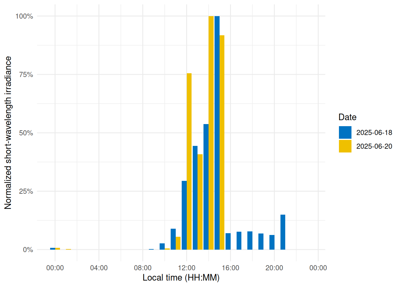
To visualize short-wavelength exposure over the course of a day, we aggregate the data into hourly bins. We cut the timeline into 1-hour segments (using local time), compute the mean short-wavelength irradiance in each hour for each day. @fig-shorttime shows the resulting diurnal profile, with short-wavelength exposure expressed as a fraction of the daily maximum for easier comparison.
```{r}
#| label: fig-shorttime
#| filename: Plot a diurnal profile
#| fig-cap: "Diurnal profile of short-wavelength light exposure. Each bar represents the average short-wavelength irradiance at that hour of the day (0–23 h), normalized to the daily maximum."
dataVEETtime <- dataVEET |> #<1>
cut_Datetime(unit = "1 hour", type = "floor", group_by = TRUE) |> #<2>
select(-c(Spectrum, long, Datetime)) |>
summarize_numeric(prefix = "") |>
add_Time_col(Datetime.rounded) |> # <3>
mutate(rel_short = short / max(short))
dataVEETtime |> #<4>
ggplot(aes(x=Time, y = rel_short)) +
geom_col(aes(fill = factor(Date)), position = "dodge") +
ggsci::scale_fill_jco() +
theme_minimal() +
labs(y = "Normalized short-wavelength irradiance",
x = "Local time (HH:MM)",
fill = "Date") +
scale_y_continuous(labels = scales::label_percent()) +
scale_x_time(labels = scales::label_time(format = "%H:%M"))
```
1. Prepare hourly binned data
2. Bin timestamps by hour
3. Add a Time column (hour of day)
4. Creating the plot
```{r}
#| echo: false
#| output: false
ggsave("manuscript/figures/Figure11.pdf",
device = cairo_pdf,
width = 5,
height = 4)
```
##### Day vs. night (photoperiod)
Finally, we compare short-wavelength exposure during daytime vs. nighttime. Using civil dawn and dusk information (based on geographic coordinates, here set for Houston, TX, USA), we label each measurement as day or night and then compute the total short-wavelength exposure in each period. @tbl-daytime summarizes the daily short-wavelength dose received during the day vs. during the night.
```{r}
#| label: tbl-daytime
#| filename: Calculate photoperiod dependent measures
#| tbl-cap: "Short wavelength light exposure (mW/m²) during the day and at night"
dataVEET |>
  select(-c(Spectrum, long, `sl ratio`, melEDI, illuminance)) |>
  add_photoperiod(coordinates) |>
  group_by(photoperiod.state, .add = TRUE) |>
  summarize_numeric(prefix = "",
                    remove = c("dawn", "dusk", "photoperiod", "Datetime")) |>
  group_by(Id, photoperiod.state) |>
  select(-episodes) |>
  pivot_wider(names_from =photoperiod.state, values_from = short) |>
  gt() |>
  fmt_number(scale_by = 1000, decimals = 1) |>
    spanner(c(day, night), "Irradiance mW/m²") |>
  cols_label_with(fn = str_to_sentence)
```
::: callout-note
In the code cell above, `add_photoperiod(coordinates)` is used as a convenient way to add columns to the data frame, indicating for each timestamp whether it was day or night, given the latitude/longitude.
:::
::::
## Discussion and conclusion
This tutorial demonstrates a standardized, step-by-step pipeline to calculate a variety of visual experience metrics. We illustrated how a combination of LightLogR functions and tidyverse workflows can yield clear and reproducible analyses for wearable device data. While the full pipeline is detailed, each metric is computed through a dedicated sequence of well-documented steps, yet remains configurable to realize different metric definitions or thresholds.
By leveraging LightLogR’s framework alongside common data analysis approaches, the process remains transparent and relatively easy to follow. The overall goal is to make analysis transparent (with open-source functions), accessible (through thorough documentation, tutorials, and human-readable function naming, all under an MIT license), robust (the package includes \>900 unit tests and continuous integration with bug tracking on GitHub), and community-driven (open feature requests and contributions via GitHub).
Even with standardized pipelines, researchers must still make and document many decisions during data cleaning, time-series handling, and metric calculations — especially for complex metrics that involve grouping data in multiple ways (for example, grouping by distance range as well as by duration for cluster metrics). We have highlighted these decision points in the tutorial (such as how to handle irregular intervals, choosing thresholds for “near” distances or “outdoor” light, and deciding on minimum durations for sustained events). Explicitly considering and reporting these choices is important for reproducibility and for comparing results across studies.
As with any behavior-dependent data source, light and distance measurements show substantial interindividual variability, which can lead to marked differences at the individual level. However, the overall processing pipeline generally remains unchanged when applied to group-level analyses. Metric parameters may still require adjustment, particularly when they are determined by device-specific sensor constraints rather than theoretical considerations. For example, the operational definition of near work may vary across populations and devices.
Another important consideration is the role of contextual data in disentangling light and distance patterns into their contributing factors beyond time of day alone. This often requires data sources in addition to the wearable device itself, such as logs or diaries. @zauner2026 describe a strategy for collecting multiple auxiliary data modalities, including activity, sleep, wear time, and other relevant measures. LightLogR provides functions to annotate wearable datasets with such contextual information, enabling more detailed analyses of visual experience data in relation to behaviour and environmental context. A [free interactive online training course](https://tscnlab.github.io/LightLogR_webinar/) for the package highlights these advanced analytical pipelines and provides specific examples.
The broad set of features in LightLogR — ranging from data import and cleaning tools (for handling time gaps and irregularities) to visualization functions and metric calculators — make it a powerful toolkit for visual experience research. Our examples spanned circadian-light metrics and myopia-related metrics, demonstrating the versatility of a unified analysis approach. By using community-supported tools and workflows, researchers in vision science, chronobiology, myopia, and related fields can reduce time spent on low-level data wrangling and focus more on interpreting results and advancing scientific understanding.
## Session info {#sessioninfo}
```{r}
sessionInfo()
```
## Statements
### Acknowledgement
We thank George Hatoun and David Sullivan (Reality Labs Research) for reviewing a draft of the tutorial manuscript and providing sample data for the `VEET` for spectral analyses.
### Data availability statement
All data and code in this tutorial and Supplement 1 are available from the GitHub repository: https://github.com/tscnlab/ZaunerEtAl_JVis_2026/, archived on Zenodo: https://doi.org/10.5281/zenodo.16566014 under a MIT license (data under CC-BY license).
### Funding statement
JZ's position is funded by the MeLiDos project. The project has received funding from the European Partnership on Metrology (22NRM05 MeLiDos), co-financed from the European Union’s Horizon Europe Research and Innovation Programme and by the Participating States. Views and opinions expressed are however those of the author(s) only and do not necessarily reflect those of the European Union or EURAMET. Neither the European Union nor the granting authority can be held responsible for them. JZ, LAO, and MS received research funding from Reality Labs Research. The funders had no role in study design, data collection and analysis, decision to publish or preparation of the manuscript.
### Conflict of interest statement
JZ declares the following potential conflict of interest in the past five years (2021-2025). Funding: Received research funding from Reality Labs Research.
AN declares the following potential conflicts of interest in the past five years (2021-2025). none
LAO declares the following potential conflict of interest in the past five years (2021-2025). Consultancy: Zeiss, Alcon, EssilorLuxottica; Research support: Topcon, Meta, LLC; Patents: US 11375890 B2
MS declares the following potential conflicts of interest in the past five years (2021–2025). Academic roles: Member of the Board of Directors, Society of Light, Rhythms, and Circadian Health (SLRCH); Chair of Joint Technical Committee 20 (JTC20) of the International Commission on Illumination (CIE); Member of the Daylight Academy; Chair of Research Data Alliance Working Group Optical Radiation and Visual Experience Data. Remunerated roles: Speaker of the Steering Committee of the Daylight Academy; Ad-hoc reviewer for the Health and Digital Executive Agency of the European Commission; Ad-hoc reviewer for the Swedish Research Council; Associate Editor for LEUKOS, journal of the Illuminating Engineering Society; Examiner, University of Manchester; Examiner, Flinders University; Examiner, University of Southern Norway. Funding: Received research funding and support from the Max Planck Society, Max Planck Foundation, Max Planck Innovation, Technical University of Munich, Wellcome Trust, National Research Foundation Singapore, European Partnership on Metrology, VELUX Foundation, Bayerisch-Tschechische Hochschulagentur (BTHA), BayFrance (Bayerisch-Französisches Hochschulzentrum), BayFOR (Bayerische Forschungsallianz), and Reality Labs Research. Honoraria for talks: Received honoraria from the ISGlobal, Research Foundation of the City University of New York and the Stadt Ebersberg, Museum Wald und Umwelt. Travel reimbursements: Daimler und Benz Stiftung. Patents: Named on European Patent Application EP23159999.4A (“System and method for corneal-plane physiologically-relevant light logging with an application to personalized light interventions related to health and well-being”). With the exception of the funding source supporting this work, M.S. declares no influence of the disclosed roles or relationships on the work presented herein.
### Statement of generative AI and AI-assisted technologies in the writing process
The authors used ChatGPT during the preparation of this work. After using this tool, the authors reviewed and edited the content as needed and take full responsibility for the content of the publication.
Use of AI in contributor roles [^2]: Conceptualization: no Data curation: no Formal analysis: bug fixing Methodology: no Software: bug fixing Validation: no Visualization: tweaking of options Writing – original draft: abstract refinement Writing – review & editing: improve readability and language
[^2]: Based on the CRediT taxonomy. Funding acquisition, investigation, project administration, resources, and supervision were deemed irrelevant in this context and thus removed.
## References