Descriptive tables and figures

Study sample, light exposure distributions, and temporal context

The near-eye measurements provide the primary description of personal light exposure. Chest measurements provide a complementary description. They are summarised separately throughout.

Libraries and prepared inputs

The preparation pages supply screened minute records, metric grids, participant information, diary windows, and solar context. Shared functions implement the specified summaries and figure styling; the calculations are called below in the order that their results are used.

library(dplyr)

Attaching package: 'dplyr'

The following objects are masked from 'package:stats':

    filter, lag

The following objects are masked from 'package:base':

    intersect, setdiff, setequal, union

library(tidyr)
library(readr)
library(ggplot2)
library(gt)
if (!requireNamespace("rnaturalearthdata", quietly = TRUE)) {
  stop("Restore the project library with renv::restore(); the local Natural Earth map data are required.")
}
source("scripts/project.R")
analysis_setup()
root <- getOption("nh.root")
source("scripts/pipeline/paths_io.R")
source("scripts/pipeline/assertions.R")
source("scripts/pipeline/site_solar_context.R")
source("scripts/descriptives/descriptive_contract.R")
configure_descriptive_site_display(root)
source("scripts/descriptives/build_descriptive_data.R")
source("scripts/descriptives/build_descriptive_displays.R")
source("scripts/descriptives/build_publication_tables.R")
source("scripts/descriptives/plot_descriptive_figures.R")
source("scripts/descriptives/plot_descriptive_displays.R")
source("scripts/descriptives/sample_counts.R")
paths <- descriptive_paths(root)
for (path in paths[-1]) dir.create(path, recursive = TRUE, showWarnings = FALSE)

Astronomical context and input validation

Calculate civil-photoperiod bounds across the 2025 calendar year at absolute latitudes from 0 to 60 degrees. These bounds provide context for the observed collection dates; they do not depend on fitted models.

span_photoperiod <- tibble::tibble(
  Datetime = as.POSIXct("2025-01-01", tz = "UTC") +
    as.difftime(0:364, units = "days")
)
photoperiod_bounds <- dplyr::bind_rows(lapply(0:60, function(latitude) {
  values <- LightLogR::extract_photoperiod(
    span_photoperiod,
    c(latitude, 0)
  )
  tibble::tibble(
    absolute_latitude_deg = latitude,
    minimum_possible_photoperiod_hours = min(
      as.numeric(values$photoperiod),
      na.rm = TRUE
    ),
    maximum_possible_photoperiod_hours = max(
      as.numeric(values$photoperiod),
      na.rm = TRUE
    ),
    calendar_year = 2025L,
    solar_depression_deg = 6
  )
}))


inputs <- load_descriptive_inputs(root, photoperiod_bounds)
validate_descriptive_inputs(inputs)
write_descriptive_csv(photoperiod_bounds, file.path(paths$source_dir, "photoperiod_latitude_bounds.csv"))
photoperiod_bounds |> filter(absolute_latitude_deg %% 10 == 0) |> gt()

absolute_latitude_deg	minimum_possible_photoperiod_hours	maximum_possible_photoperiod_hours	calendar_year	solar_depression_deg
0	12.797037	12.87642	2025	6
10	12.303848	13.47885	2025	6
20	11.724468	14.16231	2025	6
30	11.094229	14.99520	2025	6
40	10.347408	16.11290	2025	6
50	9.357244	17.86095	2025	6
60	7.797164	22.42424	2025	6

Participants, collection dates, and coverage

Summarise the complete roster and the screened samples separately. Paired counts are calculated from participant-days observed at both sensor positions.

collection_days <- build_collection_days(inputs)
available_collection_days <- build_available_collection_days(inputs)
site_sample <- build_site_sample_characteristics(inputs, collection_days, available_collection_days)
participant_characteristics <- build_participant_characteristics(inputs)
participant_table_data <- build_participant_site_display(inputs, site_sample, available_collection_days)
participant_manuscript_table_data <- participant_site_manuscript_data(participant_table_data)
sample_contract <- build_sample_count_contract(inputs)
site_display <- descriptive_site_display_registry()
write_descriptive_csv(sample_contract, file.path(paths$table_dir, "sample_counts.csv"))
sample_contract |> gt()

step	placement	participants	participant_days	one_minute_real_observations
Available normalized participant metadata	participant roster	191	NA	NA
At least 80% complete before all-zero screen	near_eye	NA	818	NA
Exact all-zero days excluded	near_eye	NA	2	NA
Main dataset after all-zero screen	near_eye	141	816	1175160
At least 80% complete before all-zero screen	chest	NA	905	NA
Exact all-zero days excluded	chest	NA	3	NA
Main dataset after all-zero screen	chest	154	902	1298880
Paired main subset	paired	112	643	NA

Light metrics and daily profiles

Derive metric summaries with their analysis-specific denominators and circular timing summaries. The MDER calculation uses the explained alternative baseline and viable minute-ratio support. Profile summaries use the screened minute measurements.

metric_values <- build_metric_values(inputs)
metric_summary <- build_metric_summary(metric_values)
metric_plot_values <- build_metric_plot_values(metric_values)
metric_table_data <- build_metric_display(metric_summary)
profiles <- build_profile_sources(inputs)
recommendation <- build_recommendation_context(inputs)
recommendation_table_data <- build_recommendation_display(recommendation)
metric_summary |> select(placement, metric_id, n_participants, n_participant_days, n_observations) |> head()

# A tibble: 6 × 5
  placement metric_id           n_participants n_participant_days n_observations
  <chr>     <chr>                        <int>              <dbl>          <int>
1 near_eye  thirty_minute_arit…            141                816          37756
2 near_eye  thirty_minute_arit…             13                 78           3619
3 near_eye  thirty_minute_arit…             13                 78           3596
4 near_eye  thirty_minute_arit…             18                107           4959
5 near_eye  thirty_minute_arit…             26                150           6900
6 near_eye  thirty_minute_arit…             10                 60           2758

Sources for the illustrative figures

The seven-participant illustration uses the local alternative-preprocessing baseline and recomputes duration above 250 lx from the displayed daytime samples. The world map comes from the installed Natural Earth data package.

time_series <- build_time_series_display_sources(root)
latitude_source <- build_latitude_photoperiod_source(collection_days)
collection_counts <- build_collection_date_counts(available_collection_days)
collection_intervals <- build_collection_intervals(available_collection_days, pause_days = 6L)
protocol_flow <- build_protocol_flow(inputs, collection_days)
site_locations <- build_site_location_source(inputs)
world_map <- build_world_map_source()
figure_alt <- build_display_figure_alt_text(site_sample, metric_summary, time_series, latitude_source)
time_series$selected |> gt()

site	NA	Date	study_day	protocol_day	weekday	selection_rule	duration_above_250_daytime_h	finite_daytime_samples	samples_above_250	participant_order
MPI	MPI_S226	2023-11-01	2	1	Wed	Seven fixed example participants and study days 2–6; displayed 30-minute values come directly from the gap-timing-unaware dataset	0.0	22	0	1
MPI	MPI_S226	2023-11-02	3	2	Thu	Seven fixed example participants and study days 2–6; displayed 30-minute values come directly from the gap-timing-unaware dataset	0.5	20	1	1
MPI	MPI_S226	2023-11-03	4	3	Fri	Seven fixed example participants and study days 2–6; displayed 30-minute values come directly from the gap-timing-unaware dataset	5.0	22	10	1
MPI	MPI_S226	2023-11-04	5	4	Sat	Seven fixed example participants and study days 2–6; displayed 30-minute values come directly from the gap-timing-unaware dataset	0.0	22	0	1
MPI	MPI_S226	2023-11-05	6	5	Sun	Seven fixed example participants and study days 2–6; displayed 30-minute values come directly from the gap-timing-unaware dataset	0.0	22	0	1
BAUA	BAUA_S003	2025-06-12	2	1	Wed	Seven fixed example participants and study days 2–6; displayed 30-minute values come directly from the gap-timing-unaware dataset	0.0	36	0	2
BAUA	BAUA_S003	2025-06-13	3	2	Thu	Seven fixed example participants and study days 2–6; displayed 30-minute values come directly from the gap-timing-unaware dataset	5.5	36	11	2
BAUA	BAUA_S003	2025-06-14	4	3	Fri	Seven fixed example participants and study days 2–6; displayed 30-minute values come directly from the gap-timing-unaware dataset	2.5	36	5	2
BAUA	BAUA_S003	2025-06-15	5	4	Sat	Seven fixed example participants and study days 2–6; displayed 30-minute values come directly from the gap-timing-unaware dataset	0.0	36	0	2
BAUA	BAUA_S003	2025-06-16	6	5	Sun	Seven fixed example participants and study days 2–6; displayed 30-minute values come directly from the gap-timing-unaware dataset	0.5	36	1	2
MPI	MPI_S227	2023-11-01	2	1	Wed	Seven fixed example participants and study days 2–6; displayed 30-minute values come directly from the gap-timing-unaware dataset	1.5	22	3	3
MPI	MPI_S227	2023-11-02	3	2	Thu	Seven fixed example participants and study days 2–6; displayed 30-minute values come directly from the gap-timing-unaware dataset	1.0	22	2	3
MPI	MPI_S227	2023-11-03	4	3	Fri	Seven fixed example participants and study days 2–6; displayed 30-minute values come directly from the gap-timing-unaware dataset	2.0	20	4	3
MPI	MPI_S227	2023-11-04	5	4	Sat	Seven fixed example participants and study days 2–6; displayed 30-minute values come directly from the gap-timing-unaware dataset	0.0	22	0	3
MPI	MPI_S227	2023-11-05	6	5	Sun	Seven fixed example participants and study days 2–6; displayed 30-minute values come directly from the gap-timing-unaware dataset	0.0	20	0	3
BAUA	BAUA_S022	2025-09-25	2	1	Wed	Seven fixed example participants and study days 2–6; displayed 30-minute values come directly from the gap-timing-unaware dataset	0.0	26	0	4
BAUA	BAUA_S022	2025-09-26	3	2	Thu	Seven fixed example participants and study days 2–6; displayed 30-minute values come directly from the gap-timing-unaware dataset	4.0	26	8	4
BAUA	BAUA_S022	2025-09-27	4	3	Fri	Seven fixed example participants and study days 2–6; displayed 30-minute values come directly from the gap-timing-unaware dataset	7.0	26	14	4
BAUA	BAUA_S022	2025-09-28	5	4	Sat	Seven fixed example participants and study days 2–6; displayed 30-minute values come directly from the gap-timing-unaware dataset	7.0	26	14	4
BAUA	BAUA_S022	2025-09-29	6	5	Sun	Seven fixed example participants and study days 2–6; displayed 30-minute values come directly from the gap-timing-unaware dataset	4.0	26	8	4
MPI	MPI_S205	2023-08-30	2	1	Wed	Seven fixed example participants and study days 2–6; displayed 30-minute values come directly from the gap-timing-unaware dataset	3.5	29	7	5
MPI	MPI_S205	2023-08-31	3	2	Thu	Seven fixed example participants and study days 2–6; displayed 30-minute values come directly from the gap-timing-unaware dataset	6.5	29	13	5
MPI	MPI_S205	2023-09-01	4	3	Fri	Seven fixed example participants and study days 2–6; displayed 30-minute values come directly from the gap-timing-unaware dataset	5.0	29	10	5
MPI	MPI_S205	2023-09-02	5	4	Sat	Seven fixed example participants and study days 2–6; displayed 30-minute values come directly from the gap-timing-unaware dataset	8.0	29	16	5
MPI	MPI_S205	2023-09-03	6	5	Sun	Seven fixed example participants and study days 2–6; displayed 30-minute values come directly from the gap-timing-unaware dataset	9.0	29	18	5
TUM	TUM_S009	2024-07-17	2	1	Wed	Seven fixed example participants and study days 2–6; displayed 30-minute values come directly from the gap-timing-unaware dataset	5.5	34	11	6
TUM	TUM_S009	2024-07-18	3	2	Thu	Seven fixed example participants and study days 2–6; displayed 30-minute values come directly from the gap-timing-unaware dataset	5.0	34	10	6
TUM	TUM_S009	2024-07-19	4	3	Fri	Seven fixed example participants and study days 2–6; displayed 30-minute values come directly from the gap-timing-unaware dataset	9.5	34	19	6
TUM	TUM_S009	2024-07-20	5	4	Sat	Seven fixed example participants and study days 2–6; displayed 30-minute values come directly from the gap-timing-unaware dataset	7.0	31	14	6
TUM	TUM_S009	2024-07-21	6	5	Sun	Seven fixed example participants and study days 2–6; displayed 30-minute values come directly from the gap-timing-unaware dataset	10.0	33	20	6
BAUA	BAUA_S009	2025-06-26	2	1	Wed	Seven fixed example participants and study days 2–6; displayed 30-minute values come directly from the gap-timing-unaware dataset	6.5	35	13	7
BAUA	BAUA_S009	2025-06-27	3	2	Thu	Seven fixed example participants and study days 2–6; displayed 30-minute values come directly from the gap-timing-unaware dataset	4.5	36	9	7
BAUA	BAUA_S009	2025-06-28	4	3	Fri	Seven fixed example participants and study days 2–6; displayed 30-minute values come directly from the gap-timing-unaware dataset	9.0	36	18	7
BAUA	BAUA_S009	2025-06-29	5	4	Sat	Seven fixed example participants and study days 2–6; displayed 30-minute values come directly from the gap-timing-unaware dataset	13.5	36	27	7
BAUA	BAUA_S009	2025-06-30	6	5	Sun	Seven fixed example participants and study days 2–6; displayed 30-minute values come directly from the gap-timing-unaware dataset	12.5	36	25	7

Save numerical results and figure data

The following CSV files contain the numerical tables and exact inputs to each figure. The editable publication tables are saved automatically when displayed below.

table_outputs <- list(
  site_sample_characteristics = site_sample,
  participant_characteristics_primary = participant_characteristics,
  metric_distribution_summary = metric_summary,
  recommendation_context_near_eye = recommendation,
  participant_site_characteristics_display = participant_table_data,
  participant_site_characteristics_manuscript_display = participant_manuscript_table_data,
  metric_descriptive_summary_display = metric_table_data,
  recommendation_context_display = recommendation_table_data)
source_outputs <- list(
  collection_days = collection_days, available_collection_days = available_collection_days,
  collection_date_counts = collection_counts, collection_intervals = collection_intervals,
  protocol_flow = protocol_flow, site_locations = site_locations, world_map_wkt = world_map,
  profile_summary = profiles$profile, profile_context_bands = profiles$state,
  profile_average_periods = profiles$period, metric_plot_values = metric_plot_values,
  time_series_display_selection = time_series$selected,
  time_series_display_30_minute = time_series$series,
  time_series_display_states = time_series$states, time_series_display_metrics = time_series$metrics,
  latitude_photoperiod = latitude_source, figure_alt_text = figure_alt)
for (name in names(table_outputs)) write_descriptive_csv(table_outputs[[name]], file.path(paths$table_dir, paste0(name, ".csv")))
for (name in names(source_outputs)) write_descriptive_csv(source_outputs[[name]], file.path(paths$source_dir, paste0(name, ".csv")))

get_alt <- function(figure_id) figure_alt$short_alt_text[match(figure_id, figure_alt$figure_id)]

The study sites are displayed in the registered reader order, with country codes and fixed colours: Borås (SE), Delft (NL), Dortmund (DE), Tübingen (DE), Munich (DE), Madrid (ES), Izmir (TR), San José (CR), Kumasi (GH). The same labels, order, and colours are used throughout the tables and figures.

The normalized participant roster contains 191 participants. After the pre-specified ≥80% full-day completeness rule and exact-all-zero screen, the primary near eye dataset contains 141 participants, 816 participant-days, and 1,175,160 one-minute real observations. The complementary chest dataset contains 154 participants, 902 participant-days, and 1,298,880 one-minute real observations. The paired subset contains 112 participants and 643 participant-days.

Data coverage and measurement placements

Two of 818 otherwise eligible near eye participant-days and three of 905 otherwise eligible chest participant-days were exact-all-zero melEDI days and were excluded. A participant was not removed merely because one of their days was excluded.

sample_contract_before_gt <- sample_contract
sample_contract_key_before_gt <- sample_contract |>
  dplyr::select(step, placement)

sample_flow_display <- sample_contract |>
  dplyr::mutate(
    dplyr::across(
      c(participants, participant_days, one_minute_real_observations),
      ~ ifelse(is.na(.x), "Not applicable", format(.x, big.mark = ","))
    )
  ) |>
  dplyr::rename(
    Step = step,
    Placement = placement,
    Participants = participants,
    `Participant-days` = participant_days,
    `One-minute real observations` = one_minute_real_observations
  )

sample_flow_gt <- sample_flow_display |>
  gt::gt(rowname_col = "Step", groupname_col = "Placement") |>
  gt::cols_align(
    align = "right",
    columns = c(
      Participants,
      `Participant-days`,
      `One-minute real observations`
    )
  ) |>
  gt::tab_options(
    table.width = gt::pct(100),
    table.font.size = gt::px(12),
    container.overflow.x = "auto"
  )

stopifnot(
  inherits(sample_flow_gt, "gt_tbl"),
  identical(sample_contract, sample_contract_before_gt),
  identical(
    sample_contract |> dplyr::select(step, placement),
    sample_contract_key_before_gt
  ),
  identical(dim(sample_flow_display), c(8L, 5L))
)

sample_flow_gt

Table 1: Descriptive sample after each fixed coverage step.

	Participants	Participant-days	One-minute real observations
participant roster
Available normalized participant metadata	191	Not applicable	Not applicable
near_eye
At least 80% complete before all-zero screen	Not applicable	818	Not applicable
Exact all-zero days excluded	Not applicable	2	Not applicable
Main dataset after all-zero screen	141	816	1,175,160
chest
At least 80% complete before all-zero screen	Not applicable	905	Not applicable
Exact all-zero days excluded	Not applicable	3	Not applicable
Main dataset after all-zero screen	154	902	1,298,880
paired
Paired main subset	112	643	Not applicable

Collection dates and civil photoperiod use the union of every recorded non-all-zero participant-day across both placements. Screened-day counts retain the primary-analysis completeness rule. Declared non-wear is reported for near eye only. Participant information covers the complete normalized roster.

Main descriptive figure and table

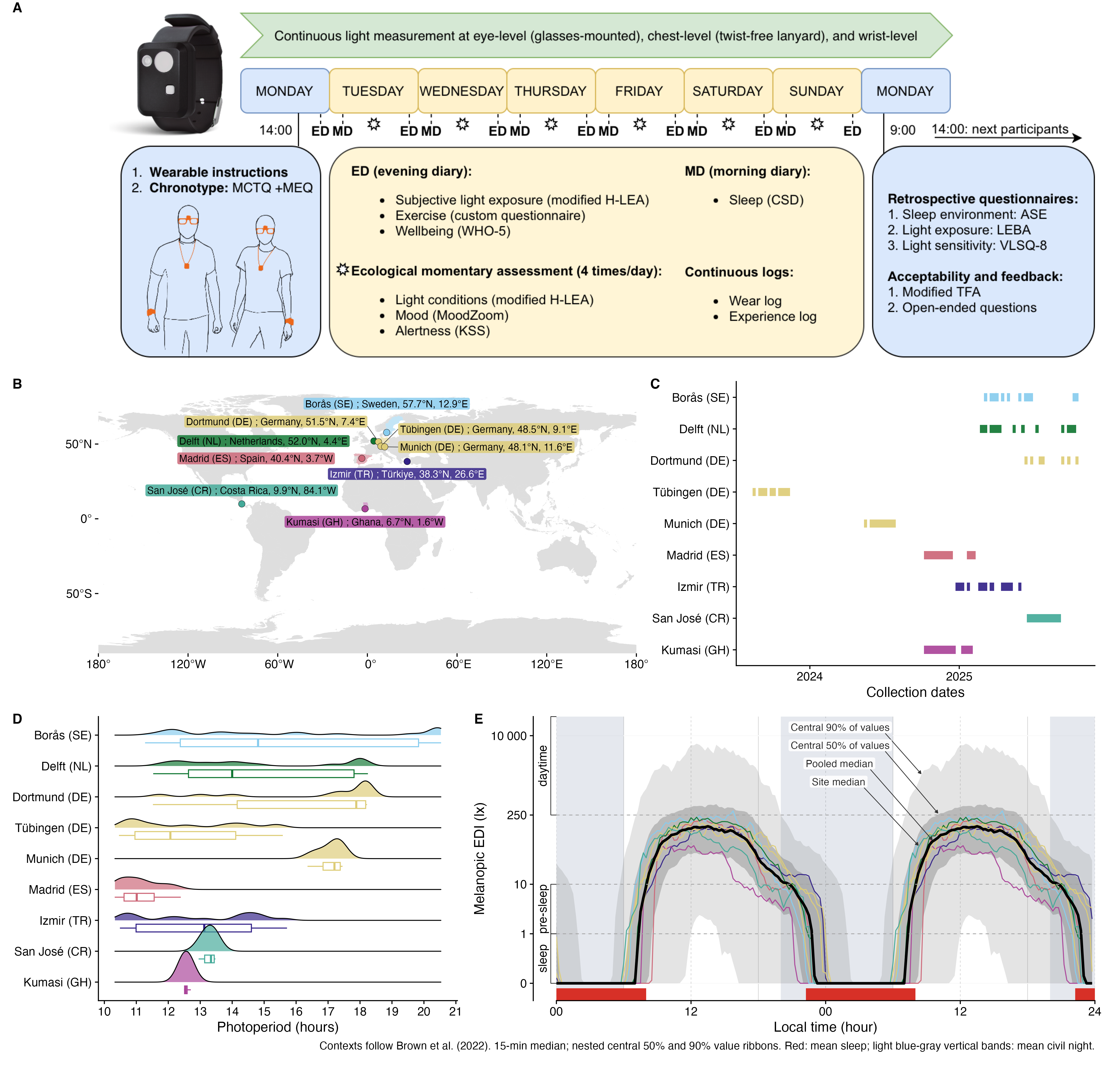
Figure 1: study overview

The five-panel overview combines the study protocol, site map, collection timing, photoperiod coverage, and a repeated 48-hour primary near eye profile. The second 24-hour cycle is a display duplicate, not additional data. Collection spans are shown as rectangles and split only when a site has at least six consecutive dates without any available data.

plot <- make_overview_display_figure(file.path(root, "assets/study-protocol.png"), site_locations, world_map, collection_intervals, available_collection_days, profiles$profile, profiles$state, profiles$period)
save_descriptive_figure(plot, file.path(paths$figure_dir, "descriptive_overview"), width = 10.5, height = 10, dpi = 300, scale = 1.5)

                                                                                                      svg 
 "/Users/zauner/Projects/ZaunerEtAl_reproducible_NH/results/images/descriptives/descriptive_overview.svg" 
                                                                                                      png 
 "/Users/zauner/Projects/ZaunerEtAl_reproducible_NH/results/images/descriptives/descriptive_overview.png" 
                                                                                                     jpeg 
"/Users/zauner/Projects/ZaunerEtAl_reproducible_NH/results/images/descriptives/descriptive_overview.jpeg" 
                                                                                                      pdf 
 "/Users/zauner/Projects/ZaunerEtAl_reproducible_NH/results/images/descriptives/descriptive_overview.pdf" 

include_project_graphics(file.path(paths$figure_dir, "descriptive_overview.png"))

Figure 1: Study protocol, country-coded sites, collection dates, observed civil photoperiod, and the pooled primary near eye 48-hour profile.

Panel B shows country and coordinate information while retaining the registered site names and colours. The black and site-coloured profiles use LightLogR::aggregate_Datetime() in 15-minute floor bins after removing participant grouping; the numeric handler is the median with na.rm = TRUE. Nested grey ribbons show the central 50% and 90% of eligible one-minute values in each overall bin, with direct arrow labels. They are value intervals, not confidence intervals. The red band from the lower plot edge to −0.1 shows average diary sleep, and blue shading shows average civil night; declared non-wear is not displayed. For the non-negative melEDI values, the symlog axis is linear from 0 to 1 lx and logarithmic above 1 lx; tick labels remain in lx. The axis is capped above 10,000 lx to reserve less space for unsupported extremes.

Table 1: participant and site characteristics

Table 2 uses site columns and identifies whether each quantity belongs to near eye, chest, paired, roster, or diary data.

participant_gt <- build_participant_site_publication_gt(participant_table_data)
participant_gt

Table 2: Participant, site, collection, sleep, chronotype, and wear characteristics.

	Overall	Borås (SE)	Delft (NL)	Dortmund (DE)	Tübingen (DE)	Munich (DE)	Madrid (ES)	Izmir (TR)	San José (CR)	Kumasi (GH)
Site specifics
Institution	Overall	RISE	THUAS	BAuA	MPI	TUM	FUSPCEU	IZTECH	UCR	KNUST
Country	Not applicable	Sweden	Netherlands	Germany	Germany	Germany	Spain	Türkiye	Costa Rica	Ghana
City	Not applicable	Borås	Delft	Dortmund	Tübingen	Munich	Madrid	Izmir	San José	Kumasi
Coordinates	Not applicable	57.7°N, 12.9°E	52.0°N, 4.4°E	51.5°N, 7.4°E	48.5°N, 9.1°E	48.1°N, 11.6°E	40.4°N, 3.7°W	38.3°N, 26.6°E	9.9°N, 84.1°W	6.7°N, 1.6°W
Data collection
Participants1	191 roster (g:143; c:157; p:116)	17 roster (g:14; c:17; p:14)	20 roster (g:13; c:15; p:13)	24 roster (g:19; c:22; p:19)	26 roster (g:26; c:0; p:0)	10 roster (g:10; c:10; p:10)	23 roster (g:23; c:22; p:22)	17 roster (g:17; c:17; p:17)	39 roster (g:6; c:39; p:6)	15 roster (g:15; c:15; p:15)
Participant-days1	1478 roster (g:1134 c:1246; p:902)	137 roster (g:107 c:137; p:107)	125 roster (g:107 c:124; p:106)	176 roster (g:145 c:163; p:132)	208 roster (g:208 c:0; p:0)	80 roster (g:80 c:80; p:80)	182 roster (g:182 c:174; p:174)	138 roster (g:138 c:138; p:138)	312 roster (g:48 c:312; p:48)	120 roster (g:119 c:118; p:117)
Weekday / weekend	g:850 / 284 c:935 / 311	g:81 / 26 c:103 / 34	g:79 / 28 c:93 / 31	g:109 / 36 c:123 / 40	g:156 / 52 c:0 / 0	g:60 / 20 c:60 / 20	g:136 / 46 c:130 / 44	g:104 / 34 c:104 / 34	g:36 / 12 c:233 / 79	g:89 / 30 c:89 / 29
Workday / free-day diaries	824 work / 451 free (n=1275 diaries)	77 work / 40 free (n=117 diaries)	70 work / 31 free (n=101 diaries)	95 work / 54 free (n=149 diaries)	115 work / 66 free (n=181 diaries)	38 work / 32 free (n=70 diaries)	95 work / 54 free (n=149 diaries)	99 work / 38 free (n=137 diaries)	180 work / 87 free (n=267 diaries)	55 work / 49 free (n=104 diaries)
Participant time2	116w 4d	11w 23h	11w 23h	15w 2d	21w 3d	8w 4d	18w 3d	14w 3d	4w 4d	11w 4d
Declared non-wear2	g:4w 1d (3.66%)	g:2d 14h (3.34%)	g:3d 1h (3.92%)	g:3d 15h (3.42%)	g:6d 10h (4.30%)	g:2d 17h (4.55%)	g:2d 20h (2.20%)	g:3d 3h (3.13%)	g:1d 11h (4.66%)	g:3d 21h (4.80%)
Screened days1,3	g:816 c:902	g:78 c:96	g:78 c:93	g:107 c:114	g:150 c:0	g:60 c:60	g:129 c:123	g:101 c:102	g:32 c:230	g:81 c:84
Collection dates4	23/08/14–25/10/20 (n=1478 d)	25/03/03–25/10/20 (n=137 d)	25/02/21–25/10/14 (n=125 d)	25/06/10–25/10/20 (n=176 d)	23/08/14–23/11/13 (n=208 d)	24/05/13–24/07/29 (n=80 d)	24/10/07–25/02/10 (n=182 d)	24/12/23–25/06/02 (n=138 d)	25/06/16–25/09/07 (n=312 d)	24/10/07–25/02/03 (n=120 d)
Civil photoperiod5,2	13.25 h (10.62–18.20) (n=1478 d)	14.81 h (11.80–20.49) (n=137 d)	14.00 h (11.88–18.09) (n=125 d)	17.88 h (11.76–18.22) (n=176 d)	12.07 h (10.55–15.41) (n=208 d)	17.20 h (16.45–17.45) (n=80 d)	11.01 h (10.35–12.22) (n=182 d)	13.13 h (10.52–15.57) (n=138 d)	13.34 h (13.01–13.47) (n=312 d)	12.54 h (12.49–12.68) (n=120 d)
Participant information
Age5	28 y (21 y–52 y) (n=191 N)	38 y (22.6 y–64.8 y) (n=17 N)	30.5 y (19.9 y–57.1 y) (n=20 N)	35.5 y (20.1 y–58.5 y) (n=24 N)	27 y (22 y–37 y) (n=26 N)	27.5 y (22.2 y–29 y) (n=10 N)	31 y (20.2 y–54.3 y) (n=23 N)	24 y (21 y–29.6 y) (n=17 N)	34 y (22 y–48.1 y) (n=39 N)	23 y (20.1 y–25 y) (n=15 N)
Sex6	F:105 / M:86 (n=191)	F:6 / M:11 (n=17)	F:8 / M:12 (n=20)	F:13 / M:11 (n=24)	F:14 / M:12 (n=26)	F:6 / M:4 (n=10)	F:15 / M:8 (n=23)	F:11 / M:6 (n=17)	F:24 / M:15 (n=39)	F:8 / M:7 (n=15)
Gender7	W:106 / M:84 / NB:1 (n=191)	W:6 / M:11 / NB:0 (n=17)	W:9 / M:10 / NB:1 (n=20)	W:13 / M:11 / NB:0 (n=24)	W:14 / M:12 / NB:0 (n=26)	W:6 / M:4 / NB:0 (n=10)	W:15 / M:8 / NB:0 (n=23)	W:11 / M:6 / NB:0 (n=17)	W:24 / M:15 / NB:0 (n=39)	W:8 / M:7 / NB:0 (n=15)
Employment status8	F:163 / P:26 / N:2 (n=191)	F:16 / P:0 / N:1 (n=17)	F:11 / P:9 / N:0 (n=20)	F:21 / P:3 / N:0 (n=24)	F:23 / P:3 / N:0 (n=26)	F:9 / P:1 / N:0 (n=10)	F:21 / P:2 / N:0 (n=23)	F:15 / P:2 / N:0 (n=17)	F:34 / P:5 / N:0 (n=39)	F:13 / P:1 / N:1 (n=15)
Chronotype group9	m:62 / i:94 / e:30 (n=186)	m:8 / i:4 / e:5 (n=17)	m:3 / i:9 / e:3 (n=15)	m:8 / i:13 / e:3 (n=24)	m:9 / i:9 / e:8 (n=26)	m:0 / i:8 / e:2 (n=10)	m:5 / i:17 / e:1 (n=23)	m:2 / i:10 / e:5 (n=17)	m:16 / i:20 / e:3 (n=39)	m:11 / i:4 / e:0 (n=15)
Sleep-corrected midsleep on free days5,10	04:03 (02:08–06:15) (n=185 N)	02:55 (02:04–05:09) (n=17 N)	04:31 (03:05–05:37) (n=15 N)	03:47 (02:17–04:49) (n=24 N)	04:33 (02:41–06:04) (n=26 N)	05:08 (04:12–06:04) (n=10 N)	04:48 (03:10–06:52) (n=22 N)	05:29 (03:35–06:49) (n=17 N)	03:42 (02:17–05:31) (n=39 N)	02:19 (01:22–03:26) (n=15 N)
Morningness–Eveningness Questionnaire score5,10	54 (35–69.8) (n=186 N)	58 (34–71.4) (n=17 N)	49 (38.4–61.3) (n=15 N)	51.5 (40.1–70.2) (n=24 N)	49 (33–68.2) (n=26 N)	44.5 (37.7–57.5) (n=10 N)	52 (42–66.8) (n=23 N)	52 (31.6–60.4) (n=17 N)	58 (40.5–69.2) (n=39 N)	62 (50.6–72.3) (n=15 N)
Social jetlag5,2	1 h (0 h–2.75 h) (n=185 N)	0.625 h (-0.0167 h–3.08 h) (n=17 N)	0.75 h (0.0875 h–1.82 h) (n=15 N)	1.27 h (0.5 h–2.16 h) (n=24 N)	0.896 h (0 h–1.85 h) (n=26 N)	0.938 h (0.5 h–2.41 h) (n=10 N)	1.38 h (0.0683 h–3.31 h) (n=22 N)	1.08 h (0.333 h–2.04 h) (n=17 N)	1.08 h (0 h–2.6 h) (n=39 N)	0.25 h (0 h–1.3 h) (n=15 N)
Sleep duration5,2	7.58 h (5.16–10.27) (n=1275 diaries / 184 N)	7.42 h (5.65–9.74) (n=117 diaries / 17 N)	7.88 h (5.75–10.00) (n=101 diaries / 15 N)	7.92 h (5.67–10.28) (n=149 diaries / 22 N)	7.43 h (4.52–9.25) (n=181 diaries / 26 N)	7.80 h (5.00–10.77) (n=70 diaries / 10 N)	7.82 h (5.87–11.67) (n=149 diaries / 23 N)	7.83 h (4.73–11.07) (n=137 diaries / 17 N)	7.08 h (5.08–9.30) (n=267 diaries / 39 N)	7.62 h (5.01–10.73) (n=104 diaries / 15 N)
1 g, near-eye glasses position; c, complementary chest position; p, paired common sample in which the same participant-day is available at both positions.
2 w: weeks; d: days; h: hours; min: minutes. Participant time and declared non-wear use eligible real minutes on screened days; both are shown for near eye only.
3 Screened days are the final participant-days after the 80% completeness screen and exclusion of exact-all-zero melEDI days.
4 Minimum–maximum local-date span across the available roster.
5 Median (5th percentile, 95th percentile).
6 Sex categories: Female and Male.
7 Gender categories: Woman, Man, and Non-binary.
8 Employment categories: Full/studying, Part/marginal, and Not employed.
9 Chronotype groups follow the Morningness–Eveningness Questionnaire score.
10 MCTQ: Munich Chronotype Questionnaire; MEQ: Morningness–Eveningness Questionnaire. Clock summaries are circular.

Reduced participant-characteristics table

The reduced participant-characteristics table provides the concise row selection used alongside the full table. It omits Morningness–Eveningness Questionnaire score, gender, collection dates, weekday/weekend counts, workday/free-day diaries, social jetlag, and sleep duration; all remaining rows retain their registered order and styling.

participant_manuscript_gt <-
  build_participant_site_manuscript_publication_gt(participant_table_data)
participant_manuscript_gt

Table 3: Reduced participant and site characteristics.

	Overall	Borås (SE)	Delft (NL)	Dortmund (DE)	Tübingen (DE)	Munich (DE)	Madrid (ES)	Izmir (TR)	San José (CR)	Kumasi (GH)
Site specifics
Institution	Overall	RISE	THUAS	BAuA	MPI	TUM	FUSPCEU	IZTECH	UCR	KNUST
Country	Not applicable	Sweden	Netherlands	Germany	Germany	Germany	Spain	Türkiye	Costa Rica	Ghana
City	Not applicable	Borås	Delft	Dortmund	Tübingen	Munich	Madrid	Izmir	San José	Kumasi
Coordinates	Not applicable	57.7°N, 12.9°E	52.0°N, 4.4°E	51.5°N, 7.4°E	48.5°N, 9.1°E	48.1°N, 11.6°E	40.4°N, 3.7°W	38.3°N, 26.6°E	9.9°N, 84.1°W	6.7°N, 1.6°W
Data collection
Participants1	191 roster (g:143; c:157; p:116)	17 roster (g:14; c:17; p:14)	20 roster (g:13; c:15; p:13)	24 roster (g:19; c:22; p:19)	26 roster (g:26; c:0; p:0)	10 roster (g:10; c:10; p:10)	23 roster (g:23; c:22; p:22)	17 roster (g:17; c:17; p:17)	39 roster (g:6; c:39; p:6)	15 roster (g:15; c:15; p:15)
Participant-days1	1478 roster (g:1134 c:1246; p:902)	137 roster (g:107 c:137; p:107)	125 roster (g:107 c:124; p:106)	176 roster (g:145 c:163; p:132)	208 roster (g:208 c:0; p:0)	80 roster (g:80 c:80; p:80)	182 roster (g:182 c:174; p:174)	138 roster (g:138 c:138; p:138)	312 roster (g:48 c:312; p:48)	120 roster (g:119 c:118; p:117)
Participant time2	116w 4d	11w 23h	11w 23h	15w 2d	21w 3d	8w 4d	18w 3d	14w 3d	4w 4d	11w 4d
Declared non-wear2	g:4w 1d (3.66%)	g:2d 14h (3.34%)	g:3d 1h (3.92%)	g:3d 15h (3.42%)	g:6d 10h (4.30%)	g:2d 17h (4.55%)	g:2d 20h (2.20%)	g:3d 3h (3.13%)	g:1d 11h (4.66%)	g:3d 21h (4.80%)
Screened days1,3	g:816 c:902	g:78 c:96	g:78 c:93	g:107 c:114	g:150 c:0	g:60 c:60	g:129 c:123	g:101 c:102	g:32 c:230	g:81 c:84
Civil photoperiod4,2	13.25 h (10.62–18.20) (n=1478 d)	14.81 h (11.80–20.49) (n=137 d)	14.00 h (11.88–18.09) (n=125 d)	17.88 h (11.76–18.22) (n=176 d)	12.07 h (10.55–15.41) (n=208 d)	17.20 h (16.45–17.45) (n=80 d)	11.01 h (10.35–12.22) (n=182 d)	13.13 h (10.52–15.57) (n=138 d)	13.34 h (13.01–13.47) (n=312 d)	12.54 h (12.49–12.68) (n=120 d)
Participant information
Age4	28 y (21 y–52 y) (n=191 N)	38 y (22.6 y–64.8 y) (n=17 N)	30.5 y (19.9 y–57.1 y) (n=20 N)	35.5 y (20.1 y–58.5 y) (n=24 N)	27 y (22 y–37 y) (n=26 N)	27.5 y (22.2 y–29 y) (n=10 N)	31 y (20.2 y–54.3 y) (n=23 N)	24 y (21 y–29.6 y) (n=17 N)	34 y (22 y–48.1 y) (n=39 N)	23 y (20.1 y–25 y) (n=15 N)
Sex5	F:105 / M:86 (n=191)	F:6 / M:11 (n=17)	F:8 / M:12 (n=20)	F:13 / M:11 (n=24)	F:14 / M:12 (n=26)	F:6 / M:4 (n=10)	F:15 / M:8 (n=23)	F:11 / M:6 (n=17)	F:24 / M:15 (n=39)	F:8 / M:7 (n=15)
Employment status6	F:163 / P:26 / N:2 (n=191)	F:16 / P:0 / N:1 (n=17)	F:11 / P:9 / N:0 (n=20)	F:21 / P:3 / N:0 (n=24)	F:23 / P:3 / N:0 (n=26)	F:9 / P:1 / N:0 (n=10)	F:21 / P:2 / N:0 (n=23)	F:15 / P:2 / N:0 (n=17)	F:34 / P:5 / N:0 (n=39)	F:13 / P:1 / N:1 (n=15)
Chronotype group7	m:62 / i:94 / e:30 (n=186)	m:8 / i:4 / e:5 (n=17)	m:3 / i:9 / e:3 (n=15)	m:8 / i:13 / e:3 (n=24)	m:9 / i:9 / e:8 (n=26)	m:0 / i:8 / e:2 (n=10)	m:5 / i:17 / e:1 (n=23)	m:2 / i:10 / e:5 (n=17)	m:16 / i:20 / e:3 (n=39)	m:11 / i:4 / e:0 (n=15)
Sleep-corrected midsleep on free days4,8	04:03 (02:08–06:15) (n=185 N)	02:55 (02:04–05:09) (n=17 N)	04:31 (03:05–05:37) (n=15 N)	03:47 (02:17–04:49) (n=24 N)	04:33 (02:41–06:04) (n=26 N)	05:08 (04:12–06:04) (n=10 N)	04:48 (03:10–06:52) (n=22 N)	05:29 (03:35–06:49) (n=17 N)	03:42 (02:17–05:31) (n=39 N)	02:19 (01:22–03:26) (n=15 N)
1 g, near-eye glasses position; c, complementary chest position; p, paired common sample in which the same participant-day is available at both positions.
2 w: weeks; d: days; h: hours; min: minutes. Participant time and declared non-wear use eligible real minutes on screened days; both are shown for near eye only.
3 Screened days are the final participant-days after the 80% completeness screen and exclusion of exact-all-zero melEDI days.
4 Median (5th percentile, 95th percentile).
5 Sex categories: Female and Male.
6 Employment categories: Full/studying, Part/marginal, and Not employed.
7 Chronotype groups follow the Morningness–Eveningness Questionnaire score.
8 MCTQ: Munich Chronotype Questionnaire; MEQ: Morningness–Eveningness Questionnaire. Clock summaries are circular.

Light distributions and temporal context

Table 2: metric distributions

Table 4 presents the registered metric categories and order, ten site columns, scaling column, and miniature distribution column. Every numerical cell states N, the number of participants, and d, the number of participant-days with a finite value. The site columns have equal widths and each median, interval, mean ± SD, and size line is kept intact. A compact line under each metric name states what the metric captures and why that construct is physiologically or health-relevant; these notes are context, not health- effect estimates from this descriptive dataset.

Duration and clock values are displayed to the nearest minute, with exact half-minute ties rounded to the even minute. Numerical CSV exports retain the full precision.

MDER is the arithmetic mean of viable one-minute melEDI / photopic illuminance ratios, with both channels finite and strictly positive. Each day is evaluated on a complete 1,440-minute local wall-clock grid and retained with at least 720 viable ratios (the inclusive 50% rule). Fall-back duplicate local minutes are averaged within channel before the ratio is formed; spring-forward absent minutes remain missing.

For the L10 mean, source windows verified as entirely zero are retained as exact 0 lx. Machine-precision residuals from the averaging calculation are not interpreted as positive exposure.

metric_gt <- build_metric_publication_gt(metric_table_data, metric_plot_values)
metric_gt

Table 4: Primary near eye melEDI metric distributions overall and by site.

Metric descriptive summary (near eye)
Metric1	Unit	Overall	Borås (SE)	Delft (NL)	Dortmund (DE)	Tübingen (DE)	Munich (DE)	Madrid (ES)	Izmir (TR)	San José (CR)	Kumasi (GH)	Scaling2	Distribution3
Duration
Time above 1,000 lx melEDI Bright-light exposure duration; relevant to daytime alerting and circadian entrainment.	HH:MM	00:41 (00:11, 01:34) 01:10 ± 01:28 N=141; d=816	01:18 (00:31, 03:24) 02:00 ± 01:54 N=13; d=78	01:18 (00:29, 02:12) 01:33 ± 01:28 N=13; d=78	01:03 (00:20, 02:32) 01:48 ± 02:14 N=18; d=107	00:40 (00:07, 01:25) 01:06 ± 01:22 N=26; d=150	00:39 (00:10, 01:46) 01:09 ± 01:18 N=10; d=60	00:27 (00:06, 00:53) 00:38 ± 00:47 N=23; d=129	00:30 (00:06, 01:04) 00:44 ± 00:51 N=17; d=101	00:19 (00:09, 00:43) 00:32 ± 00:33 N=6; d=32	00:43 (00:17, 01:14) 00:58 ± 00:57 N=15; d=81	Symlog (base 10; threshold 1)	Time above 1,000 lx melEDI distribution by site. Exact numerical summaries are in the adjacent cells.
Time above 250 lx melEDI during wake Waking time in recommended daytime light; relevant to alertness, entrainment, and subsequent sleep.	HH:MM	02:25 (00:51, 04:37) 03:00 ± 02:29 N=141; d=737	04:06 (02:30, 06:15) 04:21 ± 02:24 N=13; d=73	03:29 (02:03, 05:16) 03:39 ± 02:25 N=13; d=64	03:42 (02:05, 05:58) 04:05 ± 02:51 N=18; d=90	02:01 (00:47, 04:20) 02:52 ± 02:39 N=26; d=141	02:38 (00:55, 04:19) 02:57 ± 02:19 N=10; d=54	02:43 (00:54, 04:43) 03:02 ± 02:19 N=23; d=113	01:30 (00:41, 03:26) 02:09 ± 01:57 N=17; d=94	01:39 (00:32, 02:40) 01:48 ± 01:21 N=6; d=30	01:14 (00:25, 02:37) 01:45 ± 01:46 N=15; d=78	Symlog (base 10; threshold 1)	Time above 250 lx melEDI during wake distribution by site. Exact numerical summaries are in the adjacent cells.
Time below 10 lx melEDI before sleep Low-light time before bed; limits evening melatonin suppression and circadian delay.	HH:MM	01:53 (01:02, 02:35) 01:51 ± 01:02 N=139; d=655	02:16 (01:30, 02:39) 02:05 ± 00:53 N=13; d=67	01:50 (01:21, 02:52) 01:59 ± 00:57 N=12; d=50	01:42 (00:53, 02:17) 01:41 ± 00:58 N=18; d=84	01:52 (01:04, 02:25) 01:52 ± 01:06 N=26; d=132	01:43 (00:42, 02:32) 01:45 ± 01:10 N=10; d=52	01:43 (00:58, 02:50) 01:50 ± 01:05 N=23; d=105	01:31 (00:48, 02:15) 01:38 ± 01:00 N=17; d=82	02:16 (01:15, 02:39) 01:56 ± 01:00 N=6; d=25	02:30 (01:28, 02:52) 02:09 ± 00:57 N=14; d=58	Symlog (base 10; threshold 1)	Time below 10 lx melEDI before sleep distribution by site. Exact numerical summaries are in the adjacent cells.
Time below 1 lx melEDI during sleep Darkness during sleep; supports nocturnal melatonin and an undisturbed sleep environment.	HH:MM	07:08 (05:58, 08:15) 07:04 ± 01:57 N=141; d=778	07:08 (06:03, 08:18) 07:12 ± 01:46 N=13; d=76	07:14 (05:56, 08:06) 07:01 ± 01:50 N=13; d=68	07:08 (05:56, 08:16) 07:05 ± 01:50 N=18; d=95	06:54 (05:52, 07:46) 06:47 ± 01:30 N=26; d=150	05:52 (04:41, 07:03) 05:58 ± 01:58 N=10; d=60	08:06 (07:10, 09:10) 08:02 ± 01:57 N=23; d=118	06:45 (05:08, 08:15) 06:40 ± 02:07 N=17; d=99	06:56 (06:06, 07:36) 06:39 ± 01:43 N=6; d=31	07:31 (06:31, 09:00) 07:35 ± 02:15 N=15; d=81	Symlog (base 10; threshold 1)	Time below 1 lx melEDI during sleep distribution by site. Exact numerical summaries are in the adjacent cells.
Longest period above 250 lx melEDI Longest sustained bright-light bout; captures continuity of daytime circadian stimulation.	HH:MM	00:38 (00:17, 01:12) 00:55 ± 01:00 N=141; d=816	00:56 (00:28, 01:27) 01:12 ± 01:02 N=13; d=78	00:48 (00:23, 01:20) 01:09 ± 01:15 N=13; d=78	01:00 (00:21, 01:40) 01:20 ± 01:31 N=18; d=107	00:35 (00:13, 01:06) 00:50 ± 00:54 N=26; d=150	00:38 (00:18, 01:32) 01:01 ± 01:02 N=10; d=60	00:38 (00:16, 01:04) 00:45 ± 00:36 N=23; d=129	00:34 (00:14, 00:55) 00:43 ± 00:41 N=17; d=101	00:28 (00:16, 00:43) 00:30 ± 00:20 N=6; d=32	00:23 (00:15, 00:49) 00:38 ± 00:45 N=15; d=81	Symlog (base 10; threshold 1)	Longest period above 250 lx melEDI distribution by site. Exact numerical summaries are in the adjacent cells.
Dynamics
Interdaily stability Day-to-day regularity of the light–dark pattern; higher regularity supports circadian stability.	dimensionless	0.308 (0.248, 0.38) 0.318 ± 0.095 N=141; d=816	0.311 (0.272, 0.367) 0.315 ± 0.078 N=13; d=78	0.258 (0.239, 0.389) 0.288 ± 0.094 N=13; d=78	0.264 (0.219, 0.319) 0.274 ± 0.074 N=18; d=107	0.329 (0.263, 0.424) 0.344 ± 0.107 N=26; d=150	0.244 (0.218, 0.277) 0.252 ± 0.058 N=10; d=60	0.352 (0.321, 0.455) 0.368 ± 0.092 N=23; d=129	0.278 (0.254, 0.394) 0.323 ± 0.104 N=17; d=101	0.342 (0.315, 0.473) 0.37 ± 0.118 N=6; d=32	0.293 (0.255, 0.354) 0.299 ± 0.062 N=15; d=81	Identity	Interdaily stability distribution by site. Exact numerical summaries are in the adjacent cells.
Intradaily variability Within-day fragmentation of light exposure; higher values indicate less consolidated light–dark input.	dimensionless	1.253 (0.93, 1.502) 1.229 ± 0.389 N=141; d=816	0.997 (0.818, 1.388) 1.088 ± 0.343 N=13; d=78	1.193 (0.96, 1.389) 1.238 ± 0.345 N=13; d=78	1.182 (0.928, 1.49) 1.177 ± 0.407 N=18; d=107	1.154 (0.801, 1.442) 1.125 ± 0.354 N=26; d=150	1.48 (0.869, 1.642) 1.332 ± 0.477 N=10; d=60	1.251 (0.999, 1.497) 1.251 ± 0.413 N=23; d=129	1.359 (0.95, 1.546) 1.307 ± 0.415 N=17; d=101	1.399 (1.282, 1.483) 1.355 ± 0.256 N=6; d=32	1.324 (1.029, 1.595) 1.344 ± 0.413 N=15; d=81	Identity	Intradaily variability distribution by site. Exact numerical summaries are in the adjacent cells.
Exposure history
melEDI dose Intensity–duration-weighted melanopic exposure; summarizes cumulative non-visual retinal light input.	klx·h	4.96 (1.936, 12.313) 10.358 ± 16.216 N=141; d=761	9.296 (3.892, 21.895) 19.923 ± 27.784 N=13; d=71	10.495 (3.855, 17.395) 15.881 ± 20.395 N=13; d=74	6.751 (2.469, 14.435) 13.809 ± 23.711 N=18; d=97	3.862 (1.411, 10.217) 7.719 ± 9.847 N=26; d=137	7.11 (1.897, 15.789) 10.055 ± 11.237 N=10; d=55	3.317 (1.703, 6.29) 6.115 ± 8.79 N=23; d=125	4.35 (1.791, 10.625) 7.49 ± 8.898 N=17; d=96	2.195 (1.339, 4.117) 3.281 ± 2.573 N=6; d=30	6.045 (2.49, 14.907) 10.016 ± 10.799 N=15; d=76	Symlog (base 10; threshold 1)	melEDI dose distribution by site. Exact numerical summaries are in the adjacent cells.
Level
Mean melEDI Geometric average of daily melEDI values, including zeros; summarizes overall exposure while reducing peak influence.	lx	5.154 (2.831, 9.225) 7.587 ± 9.496 N=141; d=816	7.569 (4.55, 11.613) 9.171 ± 7.111 N=13; d=78	6.659 (4.18, 11.674) 8.274 ± 6.558 N=13; d=78	7.704 (3.081, 13.924) 12.017 ± 18.865 N=18; d=107	5.232 (3.224, 8.188) 7.221 ± 6.33 N=26; d=150	9.013 (4.011, 15.089) 12.102 ± 12.013 N=10; d=60	3.505 (1.469, 6.211) 4.166 ± 3.272 N=23; d=129	5.857 (3.726, 7.986) 7.778 ± 6.946 N=17; d=101	4.325 (3.585, 6.77) 5.248 ± 2.85 N=6; d=32	2.144 (0.744, 4.042) 3.019 ± 2.896 N=15; d=81	Symlog (base 10; threshold 1)	Mean melEDI distribution by site. Exact numerical summaries are in the adjacent cells.
Brightest 10 h mean Mean of the brightest 10 hours; reflects the strength of the main daytime light episode.	lx	110.566 (41.513, 243.212) 214.866 ± 508.56 N=141; d=816	252.689 (104.514, 461.953) 399.302 ± 518.102 N=13; d=78	175.974 (78.625, 299.106) 262.206 ± 329.201 N=13; d=78	156.184 (67.783, 339.731) 422.54 ± 1,209.616 N=18; d=107	100.057 (33.255, 209.904) 179.372 ± 241.53 N=26; d=150	130.78 (54.044, 259.726) 201.947 ± 194.042 N=10; d=60	101.102 (24.355, 218.457) 136.312 ± 134.07 N=23; d=129	83.24 (53.17, 151.786) 120.172 ± 101.545 N=17; d=101	68.143 (45.331, 132.458) 96.735 ± 72.311 N=6; d=32	46.66 (9.242, 103.175) 82.489 ± 115.07 N=15; d=81	Symlog (base 10; threshold 1)	Brightest 10 h mean distribution by site. Exact numerical summaries are in the adjacent cells.
Darkest 10 h mean Mean of the darkest 10 hours; lower values during the biological night favour melatonin preservation and sleep.	lx	0.103 (0.02, 0.253) 0.243 ± 0.513 N=141; d=816	0.08 (0.016, 0.191) 0.183 ± 0.299 N=13; d=78	0.1 (0.035, 0.23) 0.2 ± 0.332 N=13; d=78	0.14 (0.036, 0.282) 0.223 ± 0.299 N=18; d=107	0.149 (0.074, 0.309) 0.273 ± 0.465 N=26; d=150	0.325 (0.119, 0.71) 0.515 ± 0.653 N=10; d=60	0.022 (0, 0.08) 0.054 ± 0.075 N=23; d=129	0.152 (0.052, 0.481) 0.475 ± 0.882 N=17; d=101	0.133 (0.055, 0.309) 0.411 ± 1.044 N=6; d=32	0.01 (0, 0.092) 0.059 ± 0.104 N=15; d=81	Symlog (base 10; threshold 1)	Darkest 10 h mean distribution by site. Exact numerical summaries are in the adjacent cells.
Spectrum
Melanopic daylight efficacy ratio Mean of viable one-minute melEDI/illuminance ratios; indicates melanopic efficacy relative to visual light.	dimensionless	0.724 (0.643, 0.795) 0.724 ± 0.116 N=137; d=687	0.788 (0.725, 0.872) 0.796 ± 0.162 N=13; d=74	0.743 (0.699, 0.796) 0.743 ± 0.077 N=13; d=65	0.781 (0.675, 0.853) 0.768 ± 0.118 N=18; d=97	0.65 (0.592, 0.728) 0.667 ± 0.098 N=26; d=144	0.724 (0.652, 0.773) 0.72 ± 0.093 N=10; d=55	0.668 (0.629, 0.721) 0.673 ± 0.07 N=22; d=83	0.747 (0.634, 0.834) 0.735 ± 0.122 N=17; d=91	0.719 (0.661, 0.761) 0.706 ± 0.067 N=6; d=30	0.755 (0.729, 0.82) 0.758 ± 0.097 N=12; d=48	Identity	Melanopic daylight efficacy ratio distribution by site. Exact numerical summaries are in the adjacent cells.
Timing
Midpoint of the brightest 10 hours Centre time of the brightest 10 hours; indexes the main daily circadian light cue.	HH:MM clock time	13:44 (12:48, 15:00) 13:56 ± 01:51 N=141; d=816	13:16 (12:28, 14:10) 13:20 ± 01:33 N=13; d=78	14:12 (13:23, 15:18) 14:22 ± 01:51 N=13; d=78	13:52 (12:54, 15:04) 14:00 ± 01:42 N=18; d=107	13:38 (12:47, 14:44) 13:52 ± 01:42 N=26; d=150	14:54 (12:50, 16:03) 14:31 ± 02:14 N=10; d=60	13:44 (13:06, 15:20) 14:10 ± 01:51 N=23; d=129	14:10 (13:32, 15:21) 14:25 ± 01:37 N=17; d=101	12:34 (11:49, 14:02) 12:55 ± 01:44 N=6; d=32	12:49 (12:06, 13:39) 13:03 ± 01:58 N=15; d=81	Circular clock	Midpoint of the brightest 10 hours distribution by site. Exact numerical summaries are in the adjacent cells.
Midpoint of the darkest 10 hours Centre time of the darkest 10 hours; indexes the main daily darkness cue.	HH:MM clock time	02:54 (02:01, 03:50) 02:58 ± 01:41 N=141; d=816	02:02 (01:24, 02:48) 02:03 ± 01:07 N=13; d=78	02:55 (02:01, 03:28) 02:50 ± 02:05 N=13; d=78	02:32 (01:45, 03:22) 02:37 ± 01:19 N=18; d=107	03:08 (02:11, 04:10) 03:16 ± 01:34 N=26; d=150	02:37 (01:54, 04:17) 03:10 ± 02:00 N=10; d=60	03:39 (02:43, 04:34) 03:34 ± 01:49 N=23; d=129	03:31 (02:33, 04:14) 03:26 ± 01:25 N=17; d=101	01:45 (01:05, 03:01) 02:10 ± 01:27 N=6; d=32	02:33 (02:04, 03:17) 02:36 ± 01:36 N=15; d=81	Circular clock	Midpoint of the darkest 10 hours distribution by site. Exact numerical summaries are in the adjacent cells.
First light timing above 250 lx melEDI First waking bright-light exposure; morning timing can advance circadian phase and promote alertness.	HH:MM clock time	09:08 (08:02, 10:40) 09:26 ± 02:22 N=140; d=727	07:57 (06:56, 08:33) 08:03 ± 01:32 N=13; d=74	09:04 (08:18, 09:52) 09:17 ± 01:56 N=13; d=68	08:36 (07:10, 10:13) 08:45 ± 02:21 N=18; d=93	09:43 (08:13, 10:53) 09:45 ± 02:21 N=25; d=133	09:36 (07:58, 10:53) 09:39 ± 03:12 N=10; d=56	09:32 (08:40, 11:21) 10:05 ± 02:18 N=23; d=118	10:01 (09:06, 11:52) 10:26 ± 02:28 N=17; d=95	08:11 (07:26, 09:57) 08:36 ± 01:30 N=6; d=29	08:43 (08:01, 10:10) 09:19 ± 01:52 N=15; d=61	Circular clock	First light timing above 250 lx melEDI distribution by site. Exact numerical summaries are in the adjacent cells.
Last light timing above 250 lx melEDI Last bright-light exposure; later timing may delay circadian phase and sleep onset.	HH:MM clock time	18:08 (16:27, 19:42) 18:03 ± 02:36 N=141; d=687	18:41 (17:38, 19:38) 18:39 ± 01:38 N=13; d=73	18:30 (17:37, 19:59) 18:37 ± 02:08 N=13; d=62	19:34 (18:04, 20:42) 19:16 ± 02:28 N=18; d=89	17:37 (15:35, 19:09) 17:18 ± 02:44 N=26; d=121	19:50 (18:37, 20:50) 19:33 ± 02:11 N=10; d=53	17:48 (16:46, 19:19) 18:01 ± 02:21 N=23; d=106	18:45 (17:02, 19:38) 18:23 ± 02:15 N=17; d=89	15:45 (13:20, 16:38) 15:22 ± 02:38 N=6; d=28	15:54 (14:34, 17:25) 15:46 ± 02:13 N=15; d=66	Circular clock	Last light timing above 250 lx melEDI distribution by site. Exact numerical summaries are in the adjacent cells.
Mean timing of exposure above 250 lx melEDI Average bright-light timing; summarizes the phase of daily circadian stimulation.	HH:MM clock time	13:29 (12:29, 14:39) 13:31 ± 01:52 N=141; d=742	13:20 (12:29, 14:24) 13:21 ± 01:25 N=13; d=72	13:52 (13:13, 15:06) 14:02 ± 01:41 N=13; d=71	13:44 (12:28, 14:55) 13:51 ± 01:56 N=18; d=93	13:17 (12:17, 14:31) 13:24 ± 01:45 N=26; d=138	14:04 (12:58, 15:25) 14:09 ± 02:22 N=10; d=55	13:43 (12:55, 14:29) 13:47 ± 01:33 N=23; d=117	13:58 (12:54, 14:58) 14:04 ± 01:39 N=17; d=94	11:30 (10:28, 12:38) 11:26 ± 01:36 N=6; d=31	12:17 (11:04, 13:04) 12:11 ± 01:36 N=15; d=71	Circular clock	Mean timing of exposure above 250 lx melEDI distribution by site. Exact numerical summaries are in the adjacent cells.
Median (25th percentile, 75th percentile), circular or arithmetic mean ± standard deviation, N=participants; d=participant-days with a finite value for that metric.
1 The brief meaning and relevance notes describe established physiological constructs; this descriptive table does not estimate individual health effects.
2 Scaling describes the distribution column only; printed values remain on their stated scale. Symlog uses base 10 with a linear region through 1 in the stated unit; Identity is linear; Circular clock unwraps values around the metric-specific clock centre.
3 Red lines indicate site medians. Symlog and circular-clock rows are transformed only for plotting.

The table displays the metric summaries calculated above. Clock-time means and middle-50% intervals are circular, rather than treating 23:59 and 00:01 as far apart. The miniature plots are redundant visual summaries: the adjacent cells remain the authoritative values and provide the exact denominators.

Figure 2: site-specific profiles

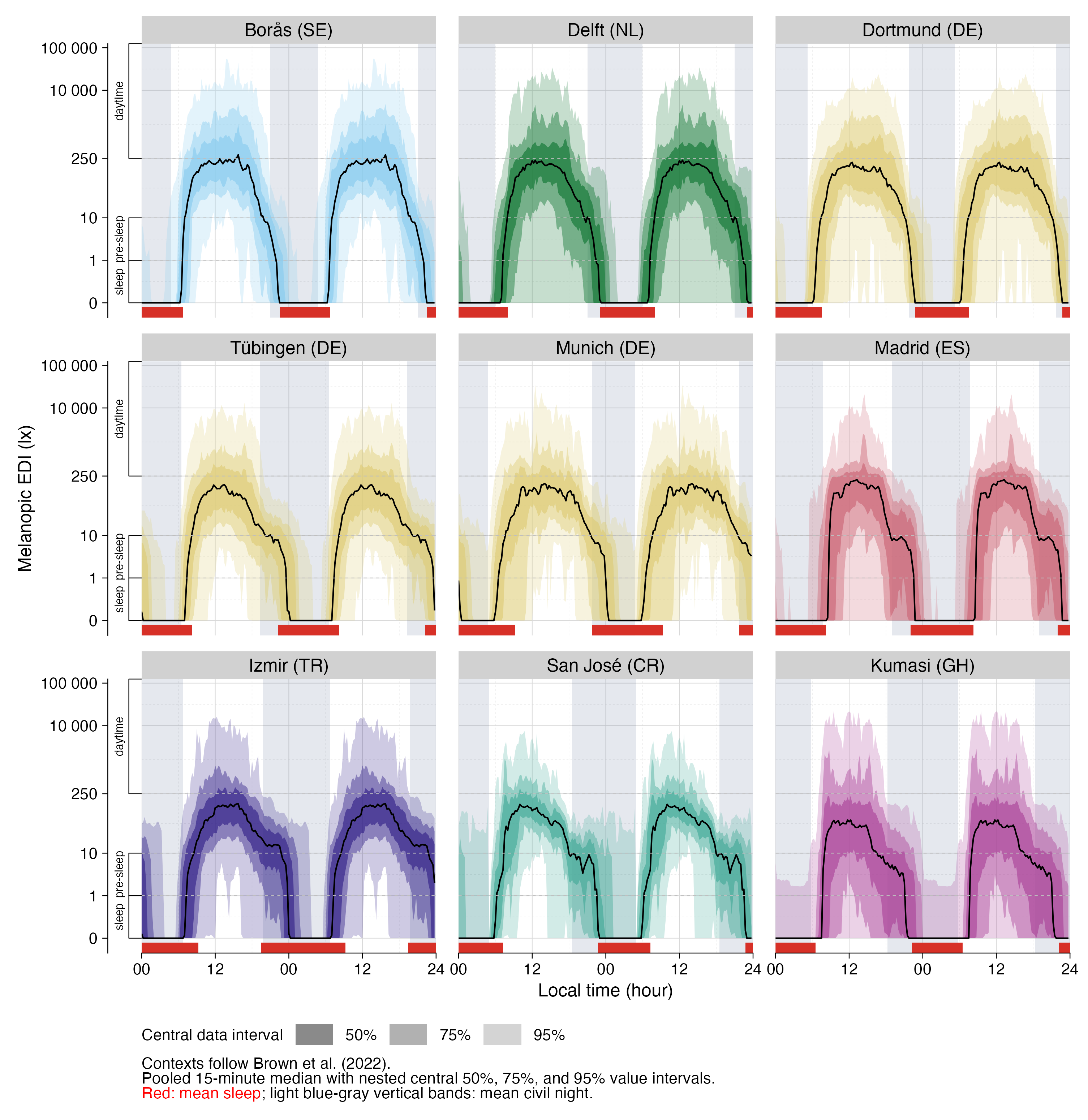
The primary near eye profiles use a 3 × 3 double-plot layout and the registered site order. Each site uses the same 15-minute aggregate_Datetime() median with nested central 50%, 75%, and 95% value intervals. The interval legend shows the corresponding ribbon opacities. The red mean-sleep strip extends from the lower plot edge to −0.1.

plot <- make_site_profile_display_figure(profiles$profile, profiles$state, profiles$period, "near_eye")
save_descriptive_figure(plot, file.path(paths$figure_dir, "near_eye_site_profiles"), width = 6.692913385826772, height = 6.889763779527559, dpi = 450, scale = 1)

                                                                                                        svg 
 "/Users/zauner/Projects/ZaunerEtAl_reproducible_NH/results/images/descriptives/near_eye_site_profiles.svg" 
                                                                                                        png 
 "/Users/zauner/Projects/ZaunerEtAl_reproducible_NH/results/images/descriptives/near_eye_site_profiles.png" 
                                                                                                       jpeg 
"/Users/zauner/Projects/ZaunerEtAl_reproducible_NH/results/images/descriptives/near_eye_site_profiles.jpeg" 
                                                                                                        pdf 
 "/Users/zauner/Projects/ZaunerEtAl_reproducible_NH/results/images/descriptives/near_eye_site_profiles.pdf" 

include_project_graphics(file.path(paths$figure_dir, "near_eye_site_profiles.png"))

Figure 2: Pooled primary near eye melEDI profiles by site, with each 24-hour cycle repeated once.

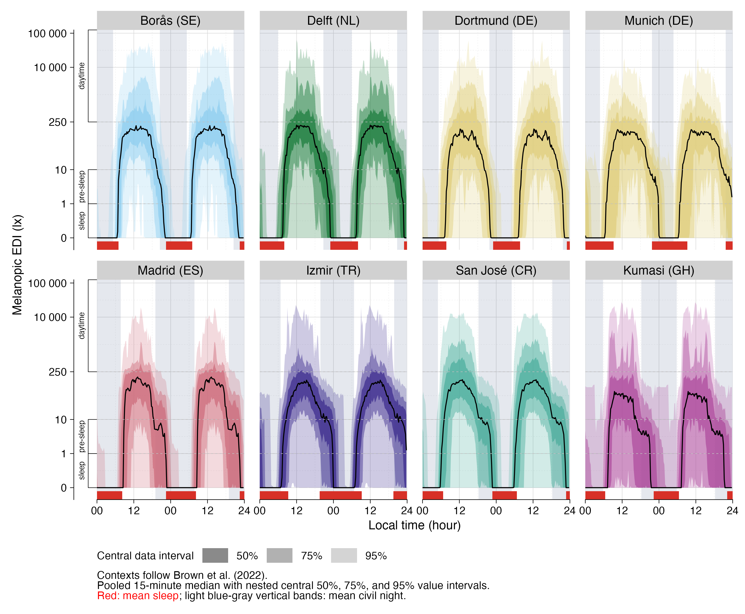
The complementary chest profile uses the same visual grammar in a complete four-by-two layout. Tübingen (DE) is omitted because the complementary chest dataset contains no eligible MPI site panel; the remaining sites retain their registered order and colours.

plot <- make_site_profile_display_figure(profiles$profile, profiles$state, profiles$period, "chest")
save_descriptive_figure(plot, file.path(paths$figure_dir, "chest_site_profiles"), width = 6.692913385826772, height = 5.511811023622047, dpi = 450, scale = 1)

                                                                                                     svg 
 "/Users/zauner/Projects/ZaunerEtAl_reproducible_NH/results/images/descriptives/chest_site_profiles.svg" 
                                                                                                     png 
 "/Users/zauner/Projects/ZaunerEtAl_reproducible_NH/results/images/descriptives/chest_site_profiles.png" 
                                                                                                    jpeg 
"/Users/zauner/Projects/ZaunerEtAl_reproducible_NH/results/images/descriptives/chest_site_profiles.jpeg" 
                                                                                                     pdf 
 "/Users/zauner/Projects/ZaunerEtAl_reproducible_NH/results/images/descriptives/chest_site_profiles.pdf" 

include_project_graphics(file.path(paths$figure_dir, "chest_site_profiles.png"))

Figure 3: Complementary chest melEDI profiles by available site, with each 24-hour cycle repeated once.

Chest values describe the environment at the chest sensor. They are not treated as equivalent to near eye or ocular exposure.

Figure 3: near eye metric distributions

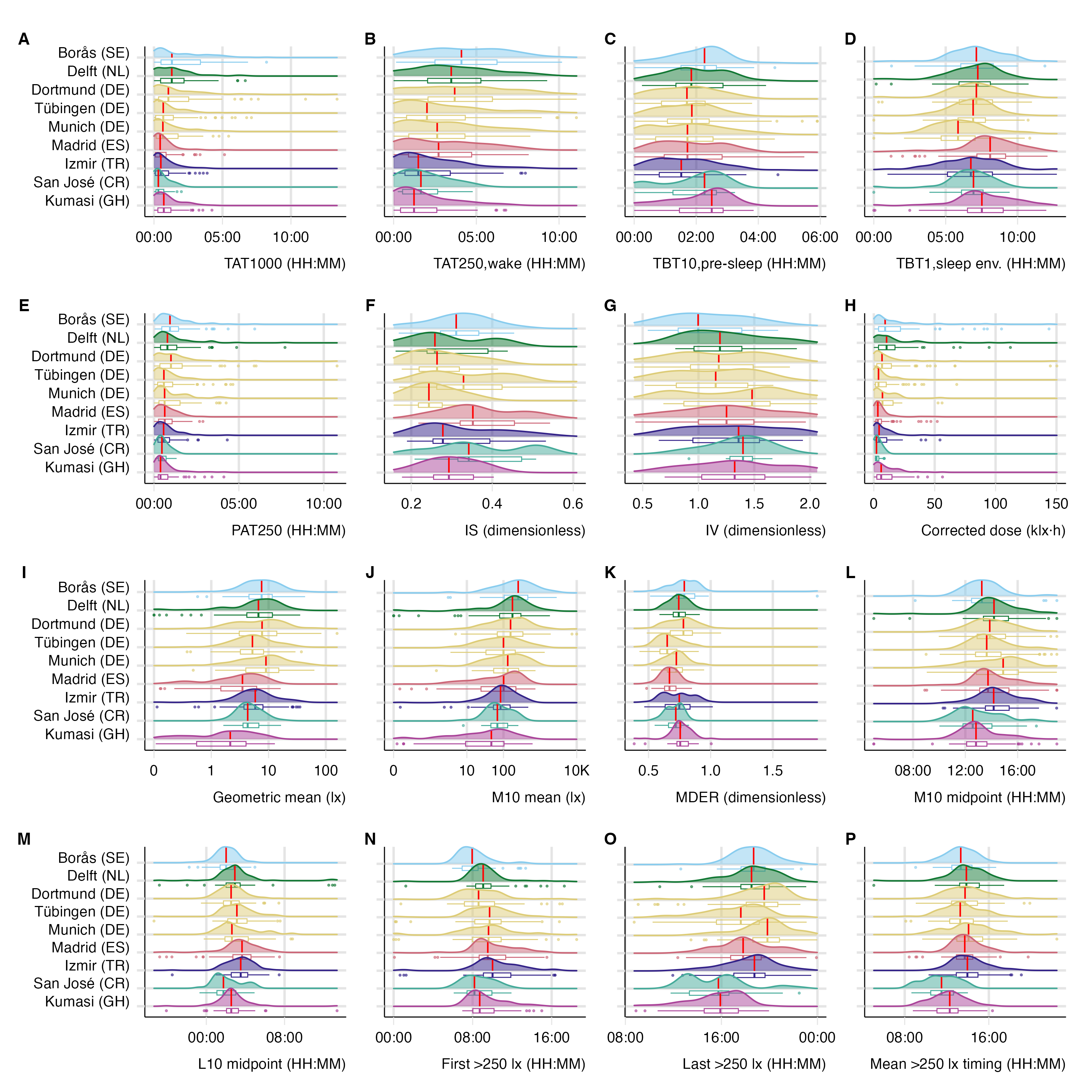
Figure 4 uses a 4 × 4 ridge-plus-box layout. Site names remain visible in the first column of panels, so colour is not the only way to identify a distribution.

plot <- make_metric_distributions_display_figure(metric_plot_values)
save_descriptive_figure(plot, file.path(paths$figure_dir, "near_eye_metric_distributions"), width = 6.692913385826772, height = 6.692913385826772, dpi = 450, scale = 1)

                                                                                                               svg 
 "/Users/zauner/Projects/ZaunerEtAl_reproducible_NH/results/images/descriptives/near_eye_metric_distributions.svg" 
                                                                                                               png 
 "/Users/zauner/Projects/ZaunerEtAl_reproducible_NH/results/images/descriptives/near_eye_metric_distributions.png" 
                                                                                                              jpeg 
"/Users/zauner/Projects/ZaunerEtAl_reproducible_NH/results/images/descriptives/near_eye_metric_distributions.jpeg" 
                                                                                                               pdf 
 "/Users/zauner/Projects/ZaunerEtAl_reproducible_NH/results/images/descriptives/near_eye_metric_distributions.pdf" 

include_project_graphics(file.path(paths$figure_dir, "near_eye_metric_distributions.png"))

Figure 4: Sixteen primary near eye melEDI metric distributions by site.

Figure 4: from time series to a daily metric

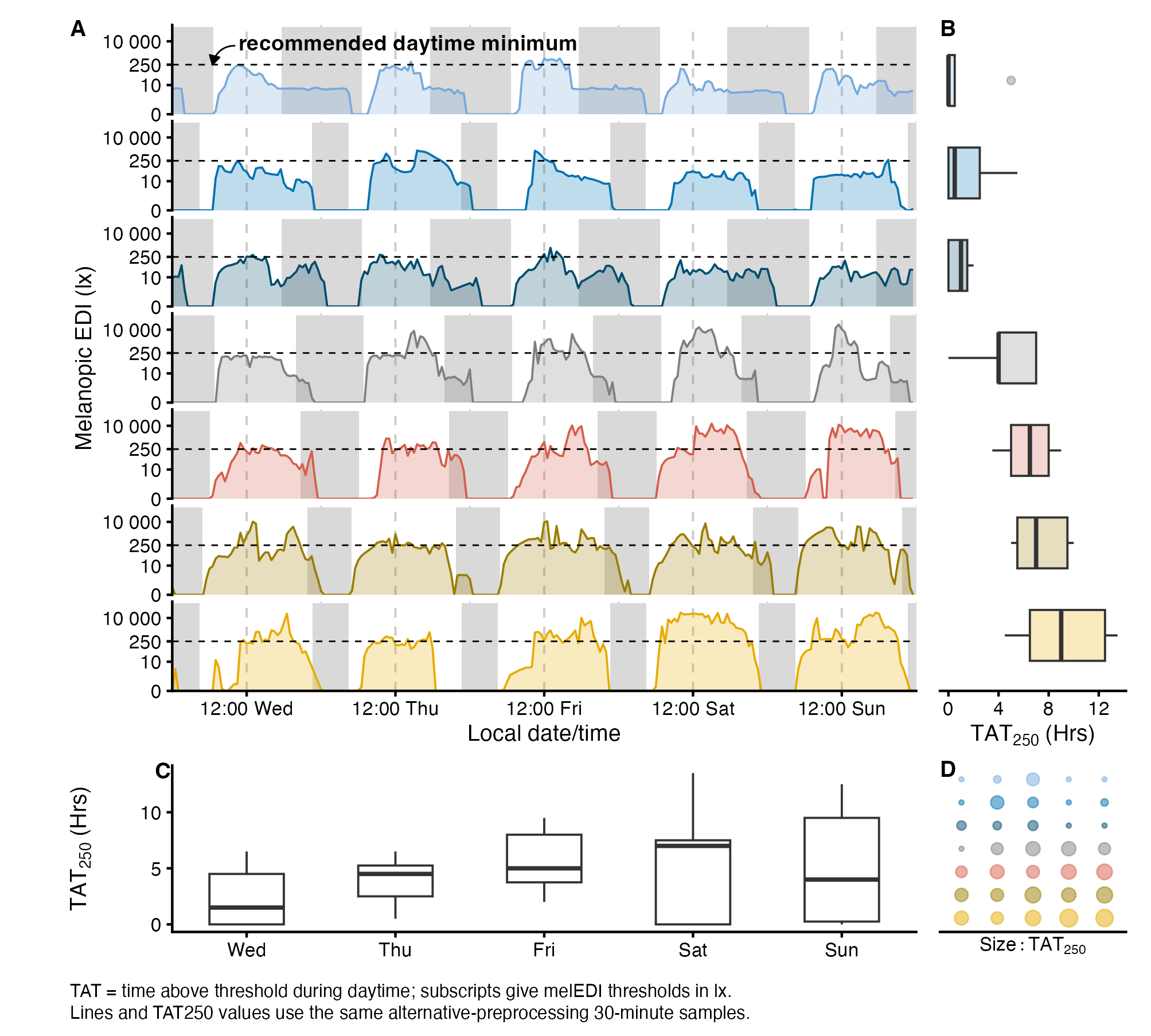
Figure 5 uses seven fixed German-site examples over five aligned study days (days 2–6) and orders participants from top to bottom by their median TAT250 across those days. The source CSV preserves each participant’s actual local dates, while the visible x-axis uses a Wednesday to Sunday alignment.

plot <- make_time_series_display_figure(time_series$series, time_series$states, time_series$metrics)
save_descriptive_figure(plot, file.path(paths$figure_dir, "time_series_to_metrics"), width = 6.692913385826772, height = 6.0236220472440944, dpi = 300, scale = 1)

                                                                                                        svg 
 "/Users/zauner/Projects/ZaunerEtAl_reproducible_NH/results/images/descriptives/time_series_to_metrics.svg" 
                                                                                                        png 
 "/Users/zauner/Projects/ZaunerEtAl_reproducible_NH/results/images/descriptives/time_series_to_metrics.png" 
                                                                                                       jpeg 
"/Users/zauner/Projects/ZaunerEtAl_reproducible_NH/results/images/descriptives/time_series_to_metrics.jpeg" 
                                                                                                        pdf 
 "/Users/zauner/Projects/ZaunerEtAl_reproducible_NH/results/images/descriptives/time_series_to_metrics.pdf" 

include_project_graphics(file.path(paths$figure_dir, "time_series_to_metrics.png"))

Figure 5: Seven fixed examples link alternative-preprocessing 30-minute near eye melEDI series to daily duration above 250 lx during daytime.

Panel A uses floor-aligned 30-minute near eye arithmetic means from the local alternative-preprocessing baseline. Panels B–D recalculate daily TAT250 from exactly those displayed daytime samples with LightLogR::duration_above_threshold(). This figure illustrates the fixed examples and does not estimate a population weekday effect.

Figure 5: latitude and observed photoperiod

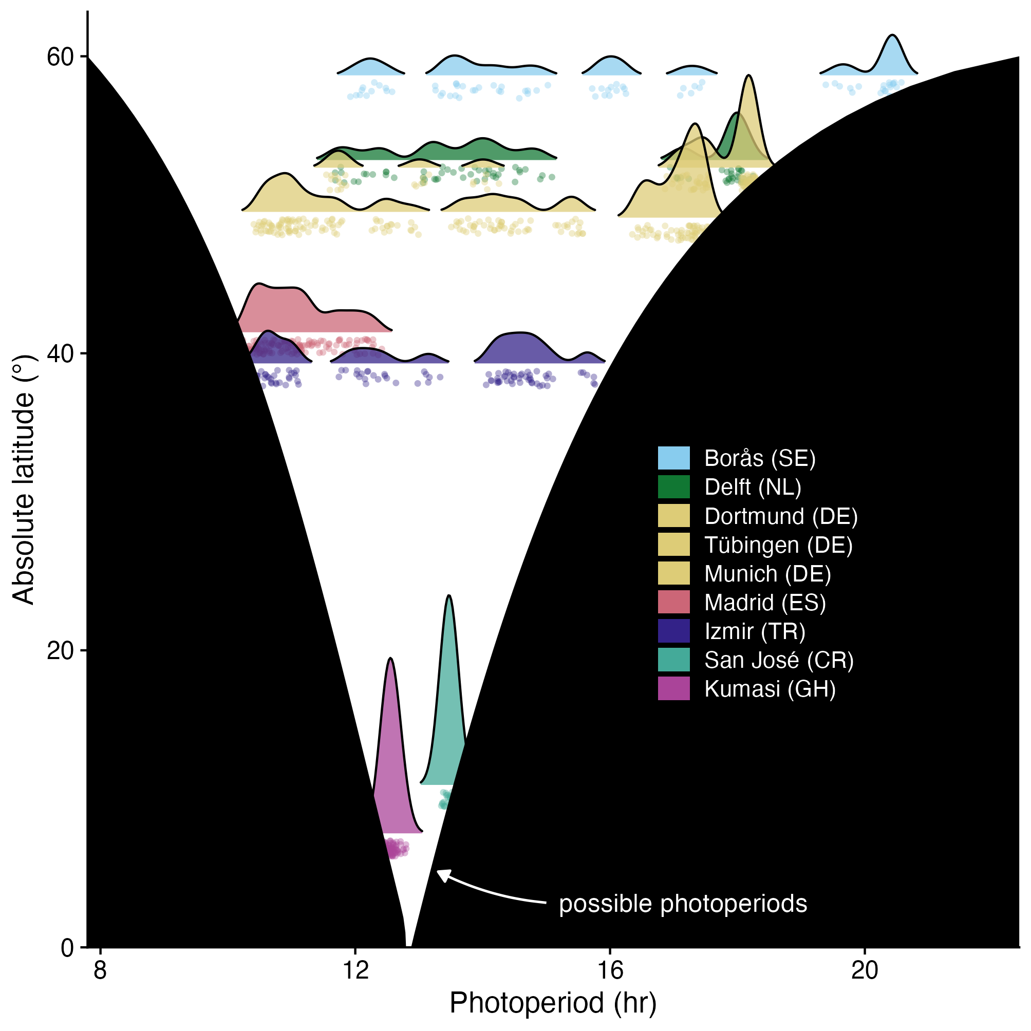
The latitude–photoperiod figure provides supplementary context for the 816 primary near eye participant-days. Black ribbons mark civil-photoperiod combinations outside the site-specific theoretical bounds. The density curves and observations are drawn first and the black feasibility curtains are drawn over them. Points use deterministic two-dimensional jitter to avoid artificial bands without changing any underlying photoperiod or latitude.

plot <- make_latitude_photoperiod_display_figure(latitude_source, photoperiod_bounds)
save_descriptive_figure(plot, file.path(paths$figure_dir, "latitude_photoperiod_diagnostic"), width = 6.692913385826772, height = 6.692913385826772, dpi = 300, scale = 1)

                                                                                                                 svg 
 "/Users/zauner/Projects/ZaunerEtAl_reproducible_NH/results/images/descriptives/latitude_photoperiod_diagnostic.svg" 
                                                                                                                 png 
 "/Users/zauner/Projects/ZaunerEtAl_reproducible_NH/results/images/descriptives/latitude_photoperiod_diagnostic.png" 
                                                                                                                jpeg 
"/Users/zauner/Projects/ZaunerEtAl_reproducible_NH/results/images/descriptives/latitude_photoperiod_diagnostic.jpeg" 
                                                                                                                 pdf 
 "/Users/zauner/Projects/ZaunerEtAl_reproducible_NH/results/images/descriptives/latitude_photoperiod_diagnostic.pdf" 

include_project_graphics(file.path(paths$figure_dir, "latitude_photoperiod_diagnostic.png"))

Figure 6: Observed civil photoperiod and theoretical bounds by absolute latitude for primary near eye participant-days.

Light exposure in Brown et al. recommendation windows

Table 5 uses site rows and recommendation-window columns. The Brown et al. recommendation windows are Daytime ≥250 lx melanopic EDI, Pre-sleep ≤10 lx melanopic EDI, and Sleep ≤1 lx melanopic EDI¹. The results are deliberately described as fractions of valid measured minutes in a recommended range, not as adherence, compliance, or evidence of a biological response.

recommendation_gt <- build_recommendation_publication_gt(
  recommendation_table_data
)
recommendation_gt

Table 5: Fractions of primary near eye minutes in the Brown et al. recommended ranges, with explicit denominators.

Site1	Minutes in the recommended range:2				Share of all eligible real minutes:3
	Daytime	Pre-sleep	Sleep4	Total5	Wake	Pre-sleep	Sleep	Unclassified6
Overall	24.0% 137,792 / 573,712	63.3% 81,894 / 129,390	87.7% 336,052 / 383,366	51.2% 555,738 / 1,086,468	51.6% 606,215 / 1,175,160	11.9% 140,152 / 1,175,160	32.6% 383,607 / 1,175,160	3.8% 45,186 / 1,175,160
Borås (SE)	33.2% 19,225 / 57,952	69.9% 8,914 / 12,759	93.4% 33,152 / 35,489	57.7% 61,291 / 106,200	54.0% 60,642 / 112,260	12.2% 13,704 / 112,260	31.7% 35,549 / 112,260	2.1% 2,365 / 112,260
Delft (NL)	29.6% 14,760 / 49,852	66.7% 7,181 / 10,774	86.4% 29,915 / 34,621	54.4% 51,856 / 95,247	47.0% 52,755 / 112,260	10.9% 12,283 / 112,260	30.9% 34,682 / 112,260	11.2% 12,540 / 112,260
Dortmund (DE)	32.4% 22,631 / 69,900	59.6% 9,749 / 16,361	87.5% 42,829 / 48,928	55.6% 75,209 / 135,189	48.1% 74,094 / 154,080	11.3% 17,409 / 154,080	31.8% 48,928 / 154,080	8.9% 13,649 / 154,080
Tübingen (DE)	22.5% 25,082 / 111,396	61.8% 15,623 / 25,283	87.1% 61,030 / 70,029	49.2% 101,735 / 206,708	55.1% 119,150 / 216,120	12.4% 26,881 / 216,120	32.4% 70,089 / 216,120	0.0% 0 / 216,120
Munich (DE)	25.0% 10,681 / 42,685	60.6% 5,963 / 9,833	71.7% 21,485 / 29,951	46.2% 38,129 / 82,469	53.0% 45,831 / 86,400	12.3% 10,618 / 86,400	34.7% 29,951 / 86,400	0.0% 0 / 86,400
Madrid (ES)	24.2% 21,067 / 87,030	62.7% 12,766 / 20,366	95.9% 58,374 / 60,891	54.8% 92,207 / 168,287	48.4% 89,948 / 185,880	11.7% 21,684 / 185,880	32.8% 60,891 / 185,880	7.2% 13,357 / 185,880
Izmir (TR)	17.8% 12,708 / 71,562	55.1% 9,221 / 16,736	79.0% 39,936 / 50,556	44.6% 61,865 / 138,854	51.5% 74,926 / 145,440	12.3% 17,883 / 145,440	34.8% 50,556 / 145,440	1.4% 2,075 / 145,440
San José (CR)	13.8% 3,266 / 23,640	64.6% 3,124 / 4,839	87.1% 12,438 / 14,275	44.0% 18,828 / 42,754	54.9% 25,285 / 46,080	11.5% 5,320 / 46,080	31.0% 14,275 / 46,080	2.6% 1,200 / 46,080
Kumasi (GH)	14.0% 8,372 / 59,695	75.2% 9,353 / 12,439	95.5% 36,893 / 38,626	49.3% 54,618 / 110,760	54.5% 63,584 / 116,640	12.3% 14,370 / 116,640	33.2% 38,686 / 116,640	0.0% 0 / 116,640
1 Near eye participant and participant-day sample sizes are reported in the participant table; every percentage cell gives its exact minute denominator.
2 Recommended ranges follow Brown et al. (2022): Daytime ≥250 lx melanopic EDI, Pre-sleep ≤10 lx melanopic EDI, and Sleep ≤1 lx melanopic EDI. Daytime, Pre-sleep, and Sleep identify the recommendation windows. Each grey numerator/denominator gives minutes within the applicable recommendation range over all valid one-minute observations in that window. Sleep describes the bedside sleep environment.
3 Each grey numerator/denominator gives minutes in the displayed diary state over all eligible real minutes before classification by diary state or measurement availability.
4 During diary-defined sleep the bedside sensor describes the sleep environment rather than direct ocular exposure.
5 Total pools all classified valid minutes.
6 Unclassified time can result from missing diary state, missing or removed melEDI measurements, or both.

Each percentage is followed by one grey numerator/denominator count. Daytime, Pre-sleep, and Sleep cells divide minutes within the applicable recommended range by all valid one-minute observations in that recommendation window; the combined column pools all classified valid minutes. The four state-share columns divide minutes in the displayed state by all eligible real minutes. Diary-defined sleep combines the near eye sensor while awake with a bedside sensor during sleep; the Sleep window therefore describes the bedside sleep environment rather than direct ocular exposure.

Data-quality and denominator qualifications

• Participant and participant-day displays distinguish the complete roster, primary near eye, complementary chest, and paired subsets. Participant time uses the screened primary near eye basis and is limited to its two largest time units.
• Site labels follow the country-coded registry, including Tübingen (DE) for MPI and Munich (DE) for TUM.
• Screened days report the result after the completeness and all-zero screens. Civil photoperiod uses the available site-and-solar context across the whole roster.
• Declared non-wear is available for near eye only. Chest values are retained solely as complementary environmental measurements.
• Clock-time chronotype and timing summaries are circular. Recommendation-window percentages retain their displayed state-specific or eligible-minute denominators.

Reproduction outputs

results/tables/descriptives/ contains the numerical summaries; results/csv/source_data/descriptives/ contains figure data; and results/images/descriptives/ contains the rendered figures. The preparation pages explain the downloaded inputs, alignment, coverage rules, and metric derivation.

References

1.

Brown, T. M. et al. Recommendations for daytime, evening, and nighttime indoor light exposure to best support physiology, sleep, and wakefulness in healthy adults. PLOS Biology 20, e3001571 (2022).