source("scripts/project.R")
analysis_setup()
source("scripts/pipeline/paths_io.R")
source("scripts/pipeline/p_value_display.R")
source("scripts/hypotheses/H07/h07_core.R")
h07_root <- normalizePath(Sys.getenv("QUARTO_PROJECT_DIR", unset = getwd()))
h07_paths <- list(root = h07_root, models = file.path(h07_root,"results/models/H07"), figures = file.path(h07_root,"results/images/H07"), tables = file.path(h07_root,"results/tables/H07"))
invisible(lapply(h07_paths[c("models","figures","tables")], h07_dir))

suppressPackageStartupMessages({
  library(dplyr)
  library(ggplot2)
  library(gratia)
  library(mgcv)
  library(purrr)
  library(readr)
  library(stringr)
  library(tibble)
  library(tidyr)
})

h07_site_display <- readr::read_csv(
  h07_path("config", "site_display_registry.csv"),
  show_col_types = FALSE
) |>
  arrange(.data$display_order)

h07_site_levels <- h07_site_display$site

h07_metric_source_map <- tibble::tribble(
  ~metric_order, ~metric_id, ~source_column, ~source_name,
  1L, "daily_geometric_mean_medi", "daily_geometric_mean_medi_lx", "Mean",
  2L, "m10_mean_medi", "m10_mean_medi_lx", "brightest_10h_mean",
  3L, "l10_mean_medi", "l10_mean_medi_lx", "darkest_10h_mean",
  4L, "duration_above_1000", "duration_above_1000_h", "duration_above_1000",
  5L, "duration_above_250_wake", "duration_above_250_wake_h", "duration_above_250_wake",
  6L, "duration_below_10_pre_sleep", "duration_below_10_pre_sleep_h", "duration_below_10_pre-sleep",
  7L, "duration_below_1_sleep_environment", "duration_below_1_sleep_environment_h", "duration_below_1_sleep",
  8L, "longest_bout_above_250", "longest_bout_above_250_h", "period_above_250",
  9L, "dose_time_sensitive_corrected_medi", "dose_corrected_medi_lx_h", "dose"
)

h07_metric_ids <- h07_metric_source_map$metric_id

h07_metric_contract <- readr::read_csv(
  h07_path(
    "results", "intermediate/model_data", "H05", "H05_metric_registry.csv"
  ),
  show_col_types = FALSE
) |>
  filter(.data$metric_id %in% h07_metric_ids) |>
  select(-"metric_order") |>
  inner_join(h07_metric_source_map, by = "metric_id") |>
  arrange(.data$metric_order)

if (
  nrow(h07_metric_contract) != 9L ||
    !identical(h07_metric_contract$metric_id, h07_metric_ids) ||
    anyNA(h07_metric_contract$response_family)
) {
  h07_abort("The nine-metric H07 contract could not be reconstructed")
}

h07_registered_formulas <- list(
  registered_null = stats::as.formula(
    "response_value ~ s(site, bs = 're') + s(site_participant, bs = 're')"
  ),
  registered_linear_surface = stats::as.formula(
    paste0(
      "response_value ~ abs_latitude_deg * photoperiod_hours + ",
      "s(site, bs = 're') + s(site_participant, bs = 're')"
    )
  ),
  registered_tensor = stats::as.formula(
    paste0(
      "response_value ~ te(abs_latitude_deg, photoperiod_hours, ",
      "k = c(4, 5), bs = c('tp', 'tp')) + ",
      "s(site, bs = 're') + s(site_participant, bs = 're')"
    )
  ),
  registered_tensor_expanded_basis = stats::as.formula(
    paste0(
      "response_value ~ te(abs_latitude_deg, photoperiod_hours, ",
      "k = c(5, 8), bs = c('tp', 'tp')) + ",
      "s(site, bs = 're') + s(site_participant, bs = 're')"
    )
  ),
  registered_tensor_fixed_site = stats::as.formula(
    paste0(
      "response_value ~ te(abs_latitude_deg, photoperiod_hours, ",
      "k = c(4, 5), bs = c('tp', 'tp')) + site + ",
      "s(site_participant, bs = 're')"
    )
  )
)

h07_adapted_formulas <- list(
  adapted_photoperiod_linear = stats::as.formula(
    paste0(
      "response_value ~ photoperiod_hours + s(site, bs = 're') + ",
      "s(site_participant, bs = 're')"
    )
  ),
  adapted_photoperiod_smooth = stats::as.formula(
    paste0(
      "response_value ~ s(photoperiod_hours, k = 6, bs = 'tp') + ",
      "s(site, bs = 're') + s(site_participant, bs = 're')"
    )
  ),
  adapted_photoperiod_expanded_basis = stats::as.formula(
    paste0(
      "response_value ~ s(photoperiod_hours, k = 10, bs = 'tp') + ",
      "s(site, bs = 're') + s(site_participant, bs = 're')"
    )
  ),
  adapted_photoperiod_fixed_site = stats::as.formula(
    paste0(
      "response_value ~ s(photoperiod_hours, k = 6, bs = 'tp') + site + ",
      "s(site_participant, bs = 're')"
    )
  )
)

h07_formulas <- c(
  h07_registered_formulas,
  h07_adapted_formulas
)

h07_formula_registry <- tibble::tibble(
  model_id = names(h07_formulas),
  formula = vapply(
    h07_formulas,
    h07_formula_text,
    character(1)
  )
)

h07_input_paths <- c(
  primary_near_eye = h07_path(
    "results", "intermediate/model_data", "base",
    "metrics_glasses_participant_day_enriched.rds"
  ),
  primary_chest = h07_path(
    "results", "intermediate/model_data", "base",
    "metrics_chest_participant_day_enriched.rds"
  ),
  gap_metrics = h07_path(
    "results", "intermediate/model_data", "scenarios", "alternative_preprocessing",
    "participant_day_metrics.rds"
  ),
  solar_context = h07_path(
    "results", "intermediate/model_data", "context", "site_solar_context.rds"
  )
)

if (!all(file.exists(h07_input_paths))) {
  h07_abort("One or more specified H07 inputs are missing")
}

h07_main_model_ids <- c(
  "registered_null",
  "registered_linear_surface",
  "registered_tensor",
  "registered_tensor_expanded_basis",
  "registered_tensor_fixed_site",
  "adapted_photoperiod_linear",
  "adapted_photoperiod_smooth",
  "adapted_photoperiod_expanded_basis",
  "adapted_photoperiod_fixed_site"
)

h07_adapted_core_model_ids <- c(
  "registered_null",
  "adapted_photoperiod_linear",
  "adapted_photoperiod_smooth"
)


source("scripts/hypotheses/H07/h07_reporting.R")H07: Photoperiod and qualifying transitions in personal light exposure
Photoperiod models relate daily exposure metrics to the recorded range of day lengths. The primary near-eye models and complementary chest models remain separate. Numerical differentiation describes qualifying transitions in the fitted curves without claiming a biological ceiling.
Data and model guide
The metric preparation supplies nine participant-day exposure outcomes, and the analysis datasets attach civil photoperiod and site/participant identifiers. Each outcome retains its own complete sample, transform and support rules. Primary near-eye and complementary chest models are separate. Site, latitude, collection season and photoperiod overlap limit what the sampled design can distinguish.
The reported pooled photoperiod smooth is fitted with mgcv::gam() using restricted maximum likelihood, a thin-plate basis of dimension six and participant random effects nested within site. Exact formulas and response families are shown below. Latitude-by-photoperiod tensor fits assess identifiability; they do not supply the reported transition classifications.
The first derivative is evaluated on the linear-predictor scale at 100 equally spaced photoperiod values. Central finite differences use a 0.01-hour increment, with one-sided differences at the boundaries, and pointwise intervals use the unconditional covariance. A qualifying transition requires an immediately preceding positive derivative interval, followed by an interval containing zero and only zero-compatible intervals thereafter to the recorded maximum. This is a descriptive rule, not an equivalence test, simultaneous band or physiological ceiling. Expanded bases, fixed-site models, exact common samples, alternative preprocessing and leave-one-site-out fits assess stability and support limitations.
The executable sections below write fitted objects to results/models/H07/, reader tables to results/tables/H07/, and the supporting numerical and figure outputs under results/. Start with the calculations below or jump to findings and interpretation.
Inputs, formulas and measurement scales
Read the regenerated participant-day metrics, solar context and response-family definitions. The formulas below distinguish the registered latitude-by-photoperiod surface from the adapted pooled photoperiod smooth.
Fit primary and complementary models
Fit the prespecified and adapted model forms for each metric and position. Each fitted model and exact sample is saved for the following diagnostics.
long_data <- h07_load_long()

run_registry <- tibble::tribble(
  ~run_id, ~data_scenario, ~placement, ~analysis_role,
  "primary__near_eye", "primary", "near_eye", "primary",
  "primary__chest", "primary", "chest", "complementary"
)

readr::write_csv(
  h07_formula_registry,
  file.path(h07_paths$tables, "H07_formula_registry.csv")
)

readr::write_csv(
  run_registry,
  file.path(h07_paths$tables, "H07_main_run_registry.csv")
)


samples <- tibble::tibble()

diagnostics <- tibble::tibble()

tests <- tibble::tibble()

for (run_index in seq_len(nrow(run_registry))) {
  run <- run_registry[run_index, , drop = FALSE]
  for (metric_id in h07_metric_ids) {
    message(
      sprintf(
        "H07 MAIN START %s / %s at %s",
        run$run_id,
        metric_id,
        format(Sys.time(), "%Y-%m-%d %H:%M:%S")
      )
    )
    result <- h07_run_metric(
      long_data = long_data,
      run_id = run$run_id,
      data_scenario = run$data_scenario,
      placement = run$placement,
      metric_id = metric_id,
      model_ids = h07_main_model_ids
    )
    samples <- bind_rows(samples, result$sample) |>
      distinct(.data$run_id, .data$metric_id, .keep_all = TRUE)
    diagnostics <- bind_rows(diagnostics, result$diagnostics) |>
      distinct(.data$run_id, .data$metric_id, .data$model_id, .keep_all = TRUE)
    tests <- bind_rows(tests, result$tests) |>
      distinct(
        .data$run_id,
        .data$metric_id,
        .data$analysis_scope,
        .data$test_id,
        .keep_all = TRUE
      )
    readr::write_csv(
      samples,
      file.path(h07_paths$tables, "H07_main_samples.csv"),
      na = ""
    )
    readr::write_csv(
      diagnostics,
      file.path(h07_paths$tables, "H07_main_diagnostics.csv"),
      na = ""
    )
    readr::write_csv(
      tests,
      file.path(h07_paths$tables, "H07_main_tests_unadjusted.csv"),
      na = ""
    )
    message(
      sprintf(
        "H07 MAIN DONE %s / %s: %s",
        run$run_id,
        metric_id,
        paste(unique(result$diagnostics$fit_status), collapse = ", ")
      )
    )
    rm(result)
    invisible(gc())
  }
}

samples <- samples |>
  arrange(
    factor(.data$run_id, levels = run_registry$run_id),
    factor(.data$metric_id, levels = h07_metric_ids)
  )

diagnostics <- diagnostics |>
  arrange(
    factor(.data$run_id, levels = run_registry$run_id),
    factor(.data$metric_id, levels = h07_metric_ids),
    factor(.data$model_id, levels = h07_main_model_ids)
  )

tests <- tests |>
  arrange(
    factor(.data$run_id, levels = run_registry$run_id),
    factor(.data$metric_id, levels = h07_metric_ids),
    .data$analysis_scope,
    .data$test_id
  )

readr::write_csv(
  samples,
  file.path(h07_paths$tables, "H07_main_samples.csv"),
  na = ""
)

readr::write_csv(
  diagnostics,
  file.path(h07_paths$tables, "H07_main_diagnostics.csv"),
  na = ""
)

readr::write_csv(
  tests,
  file.path(h07_paths$tables, "H07_main_tests_unadjusted.csv"),
  na = ""
)

tests_adjusted <- tests |>
  left_join(
    h07_metric_contract |>
      select(
        "metric_id",
        "metric_order",
        "manuscript_name",
        "response_family",
        "response_transform",
        "effect_scale",
        "display_unit"
      ),
    by = "metric_id"
  ) |>
  group_by(.data$run_id, .data$analysis_scope, .data$test_id) |>
  arrange(.data$metric_order, .by_group = TRUE) |>
  mutate(
    planned_family_n = 9L,
    p_adjusted_BH_model = stats::p.adjust(
      .data$p_raw_model,
      method = "BH",
      n = 9L
    ),
    p_raw_release = if_else(
      .data$p_release_status == "RELEASE_CONDITIONAL_APPROXIMATE",
      .data$p_raw_model,
      NA_real_
    ),
    p_adjusted_BH_release = stats::p.adjust(
      .data$p_raw_release,
      method = "BH",
      n = 9L
    ),
    conditional_aic_support = case_when(
      is.na(.data$delta_aic_full_minus_reduced) ~ "UNAVAILABLE",
      .data$delta_aic_full_minus_reduced < -2 ~ "FULL_LOWER_BY_MORE_THAN_2",
      .data$delta_aic_full_minus_reduced <= 0 ~ "FULL_LOWER_BY_0_TO_2",
      TRUE ~ "REDUCED_LOWER"
    )
  ) |>
  ungroup() |>
  arrange(
    factor(.data$run_id, levels = run_registry$run_id),
    .data$analysis_scope,
    .data$test_id,
    .data$metric_order
  )

family_diagnostic <- tests_adjusted |>
  count(
    .data$run_id,
    .data$analysis_scope,
    .data$test_id,
    name = "observed_family_n"
  ) |>
  mutate(
    planned_family_n = 9L,
    status = if_else(.data$observed_family_n == 9L, "PASS", "FAIL")
  )

if (any(family_diagnostic$status != "PASS")) {
  h07_abort("A main H07 multiplicity family is incomplete")
}

readr::write_csv(
  tests_adjusted,
  file.path(h07_paths$tables, "H07_main_tests.csv"),
  na = ""
)

readr::write_csv(
  family_diagnostic,
  file.path(h07_paths$tables, "H07_main_family_diagnostic.csv"),
  na = ""
)

message("H07 main analysis model fitting complete")
Inspect curves and model diagnostics
Evaluate fitted curves, observed predictor support, residuals and distribution checks. Distribution simulations follow the central resampling option. Basis-dimension checks use 400 residual permutations with a fixed local seed, independent of the simulation count and preceding computations.
simulation_draws <- bootstrap_count(100L)

simulation_seed_base <- 202608060L

central_step_hours <- 0.01

normal_critical <- stats::qnorm(0.975)


main_registry <- tidyr::crossing(
  placement = c("near_eye", "chest"),
  metric_id = h07_metric_ids
) |>
  left_join(
    h07_metric_contract |>
      select("metric_id", "metric_order", "manuscript_name"),
    by = "metric_id"
  ) |>
  arrange(factor(.data$placement, levels = c("near_eye", "chest")), .data$metric_order) |>
  mutate(run_id = paste("primary", .data$placement, sep = "__"))

support_points <- tibble::tibble()

site_support <- tibble::tibble()

curve_points <- tibble::tibble()

curve_summary <- tibble::tibble()

pairwise_concurvity <- tibble::tibble()

residual_summary <- tibble::tibble()

tweedie_distribution_check <- tibble::tibble()

for (row_index in seq_len(nrow(main_registry))) {
  run <- main_registry[row_index, , drop = FALSE]
  frame <- readRDS(file.path(
    h07_paths$models,
    "frames",
    run$run_id,
    paste0(run$metric_id, ".rds")
  ))
  spec <- attr(frame, "h07_spec")
  support <- h07_support_grid(frame)
  fit_bundle <- readRDS(file.path(
    h07_paths$models,
    "fits",
    run$run_id,
    run$metric_id,
    "adapted_photoperiod_smooth.rds"
  ))
  fit <- fit_bundle$fit
  curve <- h07_population_curve(
    fit,
    frame,
    spec,
    support$photoperiod_hours
  ) |>
    left_join(support, by = "photoperiod_hours")
  identity <- tibble::tibble(
    run_id = run$run_id,
    placement = run$placement,
    metric_id = run$metric_id,
    metric_order = run$metric_order,
    manuscript_name = run$manuscript_name
  )
  support_points <- bind_rows(
    support_points,
    bind_cols(identity[rep(1L, nrow(support)), ], support)
  )
  site_support <- bind_rows(
    site_support,
    frame |>
      mutate(site = as.character(.data$site)) |>
      group_by(.data$site) |>
      summarise(
        participants = n_distinct(.data$Id),
        participant_days = n(),
        first_date = min(.data$local_date),
        last_date = max(.data$local_date),
        abs_latitude_deg = unique(.data$abs_latitude_deg),
        photoperiod_min = min(.data$photoperiod_hours),
        photoperiod_max = max(.data$photoperiod_hours),
        .groups = "drop"
      ) |>
      mutate(
        run_id = run$run_id,
        placement = run$placement,
        metric_id = run$metric_id,
        metric_order = run$metric_order,
        manuscript_name = run$manuscript_name,
        .before = 1L
      )
  )
  curve_points <- bind_rows(
    curve_points,
    bind_cols(identity[rep(1L, nrow(curve)), ], curve)
  )
  eligible_curve <- curve |>
    filter(.data$pooled_eligible)
  curve_summary <- bind_rows(
    curve_summary,
    identity |>
      mutate(
        observed_grid_min = min(curve$photoperiod_hours),
        observed_grid_max = max(curve$photoperiod_hours),
        pooled_eligible_points = nrow(eligible_curve),
        loso_eligible_points = sum(curve$loso_eligible),
        supported_grid_min = if (nrow(eligible_curve)) {
          min(eligible_curve$photoperiod_hours)
        } else {
          NA_real_
        },
        supported_grid_max = if (nrow(eligible_curve)) {
          max(eligible_curve$photoperiod_hours)
        } else {
          NA_real_
        },
        supported_response_first = if (nrow(eligible_curve)) {
          eligible_curve$response_estimate[[1L]]
        } else {
          NA_real_
        },
        supported_response_last = if (nrow(eligible_curve)) {
          eligible_curve$response_estimate[[nrow(eligible_curve)]]
        } else {
          NA_real_
        },
        supported_response_difference =
          .data$supported_response_last - .data$supported_response_first,
        supported_response_ratio = if_else(
          .data$supported_response_first > 0,
          .data$supported_response_last / .data$supported_response_first,
          NA_real_
        ),
        any_negative_point_estimate = any(curve$response_estimate < 0),
        any_negative_pointwise_lower = any(curve$response_lower_pointwise < 0),
        any_above_24_hour_point_estimate = if (spec$display_unit[[1L]] == "h") {
          any(curve$response_estimate > 24)
        } else {
          NA
        },
        support_disposition = if_else(
          sum(curve$loso_eligible) == 0L,
          "NO_LOSO_STABLE_GRID_POINT",
          "HAS_LOSO_STABLE_GRID_POINTS"
        )
      )
  )
  for (model_id in c(
    "registered_tensor",
    "adapted_photoperiod_smooth",
    "adapted_photoperiod_expanded_basis",
    "adapted_photoperiod_fixed_site"
  )) {
    model_bundle <- readRDS(file.path(
      h07_paths$models,
      "fits",
      run$run_id,
      run$metric_id,
      paste0(model_id, ".rds")
    ))
    target_pattern <- if (model_id == "registered_tensor") {
      "^te\\(abs_latitude_deg"
    } else {
      "^s\\(photoperiod_hours"
    }
    pairwise_concurvity <- bind_rows(
      pairwise_concurvity,
      h07_pairwise_concurvity(model_bundle, target_pattern) |>
        mutate(
          placement = run$placement,
          metric_order = run$metric_order,
          manuscript_name = run$manuscript_name,
          .after = "run_id"
        )
    )
  }
  residual_summary <- bind_rows(
    residual_summary,
    bind_cols(
      identity,
      h07_residual_summary(fit, frame, spec)
    )
  )
  if (identical(spec$response_family[[1L]], "tweedie_log")) {
    tweedie_distribution_check <- bind_rows(
      tweedie_distribution_check,
      bind_cols(
        identity,
        h07_tweedie_distribution_check(
          fit,
          frame,
          simulation_seed_base + 1000L + run$metric_order +
            if_else(run$placement == "chest", 100L, 0L)
        )
      )
    )
  }
  message(sprintf("H07 MAIN DIAGNOSTICS DONE %s / %s", run$run_id, run$metric_id))
  rm(frame, fit, fit_bundle, curve)
  invisible(gc())
}

eligible_support_points <- support_points |>
  group_by(.data$run_id, .data$metric_id) |>
  arrange(.data$photoperiod_hours, .by_group = TRUE) |>
  mutate(
    eligible_change = .data$loso_eligible != lag(
      .data$loso_eligible,
      default = FALSE
    ),
    support_run = cumsum(.data$eligible_change)
  ) |>
  ungroup() |>
  filter(.data$loso_eligible)

support_runs <- if (nrow(eligible_support_points) == 0L) {
  tibble::tibble(
    run_id = character(),
    placement = character(),
    metric_id = character(),
    metric_order = integer(),
    manuscript_name = character(),
    support_run = integer(),
    lower = double(),
    upper = double(),
    span_hours = double(),
    sustained_one_hour = logical()
  )
} else {
  eligible_support_points |>
    group_by(
      .data$run_id,
      .data$placement,
      .data$metric_id,
      .data$metric_order,
      .data$manuscript_name,
      .data$support_run
    ) |>
    summarise(
      lower = min(.data$photoperiod_hours),
      upper = max(.data$photoperiod_hours),
      span_hours = .data$upper - .data$lower,
      sustained_one_hour = .data$span_hours >= 1 - 1e-8,
      .groups = "drop"
    )
}

h07_write_table(support_points, "H07_main_support_grid.csv")
[1] "/Users/zauner/Projects/ZaunerEtAl_reproducible_NH/results/tables/H07/H07_main_support_grid.csv"h07_write_table(support_runs, "H07_main_support_runs.csv")[1] "/Users/zauner/Projects/ZaunerEtAl_reproducible_NH/results/tables/H07/H07_main_support_runs.csv"h07_write_table(site_support, "H07_main_site_support.csv")[1] "/Users/zauner/Projects/ZaunerEtAl_reproducible_NH/results/tables/H07/H07_main_site_support.csv"h07_write_table(curve_points, "H07_main_curve_points.csv")[1] "/Users/zauner/Projects/ZaunerEtAl_reproducible_NH/results/tables/H07/H07_main_curve_points.csv"h07_write_table(curve_summary, "H07_main_curve_summary.csv")[1] "/Users/zauner/Projects/ZaunerEtAl_reproducible_NH/results/tables/H07/H07_main_curve_summary.csv"h07_write_table(
pairwise_concurvity,
"H07_main_pairwise_concurvity.csv"
)[1] "/Users/zauner/Projects/ZaunerEtAl_reproducible_NH/results/tables/H07/H07_main_pairwise_concurvity.csv"h07_write_table(
residual_summary,
"H07_main_residual_distribution_summary.csv"
)[1] "/Users/zauner/Projects/ZaunerEtAl_reproducible_NH/results/tables/H07/H07_main_residual_distribution_summary.csv"h07_write_table(
tweedie_distribution_check,
"H07_main_tweedie_distribution_check.csv"
)[1] "/Users/zauner/Projects/ZaunerEtAl_reproducible_NH/results/tables/H07/H07_main_tweedie_distribution_check.csv"curve_plot_data <- curve_points |>
mutate(
placement_label = recode(
.data$placement,
near_eye = "Near eye ; primary",
chest = "Chest ; complementary"
),
manuscript_name = factor(
.data$manuscript_name,
levels = h07_metric_contract$manuscript_name
)
)
for (placement_value in c("near_eye", "chest")) {
plot_data <- curve_plot_data |>
filter(.data$placement == .env$placement_value)
support_subtitle <- if (any(plot_data$pooled_eligible)) {
paste(
"Blue: pooled-support estimate with pointwise 95% CI.\n",
"Grey: outside the pooled support rule."
)
} else {
paste(
"No grid point passes the pooled support rule.\n",
"All curves are grey descriptive context only."
)
}
plot <- ggplot(plot_data, aes(.data$photoperiod_hours, .data$response_estimate)) +
geom_line(colour = "#9ca3af", linewidth = 0.55) +
geom_ribbon(
data = ~ filter(.x, .data$pooled_eligible),
aes(
ymin = .data$response_lower_pointwise,
ymax = .data$response_upper_pointwise
),
inherit.aes = TRUE,
fill = "#3b82f6",
alpha = 0.18,
colour = NA
) +
geom_line(
data = ~ filter(.x, .data$pooled_eligible),
colour = "#1d4ed8",
linewidth = 0.85
) +
facet_wrap(
vars(.data$manuscript_name),
scales = "free_y",
ncol = 3,
labeller = label_wrap_gen(27)
) +
scale_x_continuous(breaks = seq(10, 20, by = 2)) +
labs(
x = "Civil photoperiod (h)",
y = "Estimated metric value",
title = unique(plot_data$placement_label),
subtitle = support_subtitle
) +
theme_minimal(base_size = 10) +
theme(
panel.grid.minor = element_blank(),
strip.text = element_text(face = "bold", size = 9),
plot.title = element_text(face = "bold", size = 14),
plot.subtitle = element_text(size = 10, margin = margin(b = 10)),
plot.title.position = "plot",
plot.margin = margin(10, 10, 10, 10),
axis.title = element_text(size = 10)
)
ggplot2::ggsave(
file.path(
h07_paths$figures,
paste0("H07_main_curves_", placement_value, ".png")
),
plot,
width = 13,
height = 10,
units = "in",
dpi = 180,
bg = "white"
)
}
message("H07 analysis main diagnostic and curve artifacts complete")Fit preprocessing and sample sensitivities
Compare common samples, alternative preprocessing, and alternative valid metric definitions. Every sensitivity keeps near-eye and chest measurements separate.
long_data <- h07_load_long()

key_columns <- c("site", "Id", "local_date")

paired_keys <- long_data |>
  filter(
    .data$data_scenario == "primary",
    .data$placement %in% c("near_eye", "chest"),
    !is.na(.data$original_value)
  ) |>
  group_by(
    .data$metric_id,
    .data$site,
    .data$Id,
    .data$local_date
  ) |>
  summarise(
    placements = n_distinct(.data$placement),
    .groups = "drop"
  ) |>
  filter(.data$placements == 2L) |>
  select(-"placements")

preparation_common_keys <- long_data |>
  filter(
    .data$data_scenario %in% c("primary", "gap_timing_unaware"),
    !is.na(.data$original_value)
  ) |>
  group_by(
    .data$placement,
    .data$metric_id,
    .data$site,
    .data$Id,
    .data$local_date
  ) |>
  summarise(
    scenarios = n_distinct(.data$data_scenario),
    .groups = "drop"
  ) |>
  filter(.data$scenarios == 2L) |>
  select(-"scenarios")


variant_map <- bind_rows(
  h07_read_variant_map(
    h07_input_paths[["primary_near_eye"]],
    "near_eye"
  ),
  h07_read_variant_map(
    h07_input_paths[["primary_chest"]],
    "chest"
  )
)

if (anyDuplicated(variant_map[c("placement", key_columns)])) {
  h07_abort("H07 metric-variant source has duplicate participant-day keys")
}

exact_period_keys <- variant_map |>
  filter(
    .data$exact_period_identifiable %in% TRUE,
    is.finite(.data$exact_period_value)
  ) |>
  select("placement", all_of(key_columns))

dose_common_keys <- variant_map |>
  filter(
    is.finite(.data$corrected_dose_value),
    is.finite(.data$observed_dose_value)
  ) |>
  select("placement", all_of(key_columns))


full_run_registry <- tibble::tribble(
  ~run_id, ~data_scenario, ~placement, ~sensitivity, ~key_rule,
  "paired__near_eye", "primary", "near_eye", "paired_common_placement", "paired",
  "paired__chest", "primary", "chest", "paired_common_placement", "paired",
  "gap_timing_unaware__near_eye", "gap_timing_unaware", "near_eye", "gap_timing_unaware", "all_available",
  "gap_timing_unaware__chest", "gap_timing_unaware", "chest", "gap_timing_unaware", "all_available",
  "prep_common_primary__near_eye", "primary", "near_eye", "preparation_exact_common", "preparation_common",
  "prep_common_primary__chest", "primary", "chest", "preparation_exact_common", "preparation_common",
  "prep_common_gap__near_eye", "gap_timing_unaware", "near_eye", "preparation_exact_common", "preparation_common",
  "prep_common_gap__chest", "gap_timing_unaware", "chest", "preparation_exact_common", "preparation_common"
)

special_run_registry <- tibble::tribble(
  ~run_id, ~data_scenario, ~placement, ~sensitivity, ~key_rule, ~metric_id, ~value_column,
  "exact_period__near_eye", "primary", "near_eye", "longest_period_exact_only", "exact_period", "longest_bout_above_250", "exact_period_value",
  "exact_period__chest", "primary", "chest", "longest_period_exact_only", "exact_period", "longest_bout_above_250", "exact_period_value",
  "dose_common_corrected__near_eye", "primary", "near_eye", "observed_dose_common_sample", "dose_common", "dose_time_sensitive_corrected_medi", NA_character_,
  "dose_common_corrected__chest", "primary", "chest", "observed_dose_common_sample", "dose_common", "dose_time_sensitive_corrected_medi", NA_character_,
  "dose_common_observed__near_eye", "primary", "near_eye", "observed_dose_common_sample", "dose_common", "dose_time_sensitive_corrected_medi", "observed_dose_value",
  "dose_common_observed__chest", "primary", "chest", "observed_dose_common_sample", "dose_common", "dose_time_sensitive_corrected_medi", "observed_dose_value"
)

run_registry <- bind_rows(
  full_run_registry |>
    mutate(
      metric_id = NA_character_,
      value_column = NA_character_,
      expected_family_n = 9L
    ),
  special_run_registry |>
    mutate(expected_family_n = NA_integer_)
)

readr::write_csv(
  run_registry,
  file.path(h07_paths$tables, "H07_sensitivity_run_registry.csv"),
  na = ""
)

key_diagnostic <- bind_rows(
  paired_keys |>
    mutate(key_set = "paired_common_placement", placement = "both"),
  preparation_common_keys |>
    mutate(key_set = "preparation_exact_common"),
  exact_period_keys |>
    mutate(metric_id = "longest_bout_above_250", key_set = "longest_period_exact_only"),
  dose_common_keys |>
    mutate(metric_id = "dose_time_sensitive_corrected_medi", key_set = "observed_dose_common_sample")
) |>
  group_by(.data$key_set, .data$placement, .data$metric_id) |>
  summarise(
    participants = n_distinct(.data$site, .data$Id),
    participant_days = n(),
    sites = n_distinct(.data$site),
    .groups = "drop"
  ) |>
  left_join(
    h07_metric_contract |>
      select("metric_id", "metric_order", "manuscript_name"),
    by = "metric_id"
  ) |>
  arrange(.data$key_set, .data$placement, .data$metric_order)

readr::write_csv(
  key_diagnostic,
  file.path(h07_paths$tables, "H07_sensitivity_key_diagnostic.csv"),
  na = ""
)


samples <- tibble::tibble()

diagnostics <- tibble::tibble()

tests <- tibble::tibble()

for (run_index in seq_len(nrow(run_registry))) {
  run <- run_registry[run_index, , drop = FALSE]
  metrics <- if (is.na(run$metric_id[[1L]])) {
    h07_metric_ids
  } else {
    intersect(run$metric_id[[1L]], h07_metric_ids)
  }
  if (length(metrics) == 0L) next
  for (metric_id in metrics) {
    message(sprintf(
      "H07 SENS START %s / %s at %s",
      run$run_id,
      metric_id,
      format(Sys.time(), "%Y-%m-%d %H:%M:%S")
    ))
    keys <- h07_keys_for_run(run, metric_id)
    if (!is.null(keys) && nrow(keys) == 0L) {
      h07_abort(
        "The specified sensitivity has no exact keys: %s / %s",
        run$run_id,
        metric_id
      )
    }
    result <- h07_run_metric(
      long_data = long_data,
      run_id = run$run_id,
      data_scenario = run$data_scenario,
      placement = run$placement,
      metric_id = metric_id,
      model_ids = h07_adapted_core_model_ids,
      keys = keys,
      value_override = h07_override_for_run(run)
    )
    samples <- bind_rows(samples, result$sample) |>
      distinct(.data$run_id, .data$metric_id, .keep_all = TRUE)
    diagnostics <- bind_rows(diagnostics, result$diagnostics) |>
      distinct(.data$run_id, .data$metric_id, .data$model_id, .keep_all = TRUE)
    tests <- bind_rows(tests, result$tests) |>
      filter(.data$analysis_scope == "adapted_photoperiod") |>
      distinct(
        .data$run_id,
        .data$metric_id,
        .data$analysis_scope,
        .data$test_id,
        .keep_all = TRUE
      )
    readr::write_csv(
      samples,
      file.path(h07_paths$tables, "H07_sensitivity_samples.csv"),
      na = ""
    )
    readr::write_csv(
      diagnostics,
      file.path(h07_paths$tables, "H07_sensitivity_diagnostics.csv"),
      na = ""
    )
    readr::write_csv(
      tests,
      file.path(h07_paths$tables, "H07_sensitivity_tests_unadjusted.csv"),
      na = ""
    )
    message(sprintf(
      "H07 SENS DONE %s / %s: %s",
      run$run_id,
      metric_id,
      paste(unique(result$diagnostics$fit_status), collapse = ", ")
    ))
    rm(result)
    invisible(gc())
  }
}

samples <- samples |>
  arrange(
    factor(.data$run_id, levels = run_registry$run_id),
    factor(.data$metric_id, levels = h07_metric_ids)
  )

diagnostics <- diagnostics |>
  arrange(
    factor(.data$run_id, levels = run_registry$run_id),
    factor(.data$metric_id, levels = h07_metric_ids),
    factor(.data$model_id, levels = h07_adapted_core_model_ids)
  )

tests <- tests |>
  arrange(
    factor(.data$run_id, levels = run_registry$run_id),
    factor(.data$metric_id, levels = h07_metric_ids),
    .data$analysis_scope,
    .data$test_id
  )

readr::write_csv(
  samples,
  file.path(h07_paths$tables, "H07_sensitivity_samples.csv"),
  na = ""
)

readr::write_csv(
  diagnostics,
  file.path(h07_paths$tables, "H07_sensitivity_diagnostics.csv"),
  na = ""
)

readr::write_csv(
  tests,
  file.path(
    h07_paths$tables,
    "H07_sensitivity_tests_unadjusted.csv"
  ),
  na = ""
)

tests_adjusted <- tests |>
  left_join(
    h07_metric_contract |>
      select(
        "metric_id",
        "metric_order",
        "manuscript_name",
        "response_family",
        "response_transform",
        "effect_scale",
        "display_unit"
      ),
    by = "metric_id"
  ) |>
  left_join(
    run_registry |>
      select("run_id", "sensitivity", "placement", "expected_family_n"),
    by = "run_id"
  ) |>
  group_by(.data$run_id, .data$analysis_scope, .data$test_id) |>
  arrange(.data$metric_order, .by_group = TRUE) |>
  mutate(
    p_adjusted_BH_model = if (is.na(first(.data$expected_family_n))) {
      rep(NA_real_, n())
    } else {
      stats::p.adjust(
        .data$p_raw_model,
        method = "BH",
        n = first(.data$expected_family_n)
      )
    },
    p_raw_release = if_else(
      .data$p_release_status == "RELEASE_CONDITIONAL_APPROXIMATE",
      .data$p_raw_model,
      NA_real_
    ),
    p_adjusted_BH_release = if (is.na(first(.data$expected_family_n))) {
      rep(NA_real_, n())
    } else {
      stats::p.adjust(
        .data$p_raw_release,
        method = "BH",
        n = first(.data$expected_family_n)
      )
    },
    conditional_aic_support = case_when(
      is.na(.data$delta_aic_full_minus_reduced) ~ "UNAVAILABLE",
      .data$delta_aic_full_minus_reduced < -2 ~ "FULL_LOWER_BY_MORE_THAN_2",
      .data$delta_aic_full_minus_reduced <= 0 ~ "FULL_LOWER_BY_0_TO_2",
      TRUE ~ "REDUCED_LOWER"
    )
  ) |>
  ungroup() |>
  arrange(
    factor(.data$run_id, levels = run_registry$run_id),
    .data$test_id,
    .data$metric_order
  )

family_diagnostic <- tests_adjusted |>
  filter(!is.na(.data$expected_family_n)) |>
  count(
    .data$run_id,
    .data$analysis_scope,
    .data$test_id,
    .data$expected_family_n,
    name = "observed_family_n"
  ) |>
  mutate(
    status = if_else(
      .data$observed_family_n == .data$expected_family_n,
      "PASS",
      "FAIL"
    )
  )

if (any(family_diagnostic$status != "PASS")) {
  h07_abort("An H07 sensitivity multiplicity family is incomplete")
}

readr::write_csv(
  tests_adjusted,
  file.path(h07_paths$tables, "H07_sensitivity_tests.csv"),
  na = ""
)

readr::write_csv(
  family_diagnostic,
  file.path(h07_paths$tables, "H07_sensitivity_family_diagnostic.csv"),
  na = ""
)

message("H07 analysis sensitivity model fitting complete")
Fit leave-one-site-out models
Refit the adapted curves while omitting each site to assess site influence within the measured geographic scope.
long_data <- h07_load_long()

placements <- c("near_eye", "chest")

registry <- tidyr::crossing(
  placement = placements,
  metric_id = h07_metric_ids
) |>
  mutate(
    main_run_id = paste("primary", .data$placement, sep = "__"),
    main_frame_path = file.path(
      h07_paths$models,
      "frames",
      .data$main_run_id,
      paste0(.data$metric_id, ".rds")
    )
  )

if (!all(file.exists(registry$main_frame_path))) {
  h07_abort("A primary H07 frame required for LOSO is missing")
}

loso_registry <- purrr::pmap_dfr(
  registry,
  function(placement, metric_id, main_run_id, main_frame_path) {
    frame <- readRDS(main_frame_path)
    tibble::tibble(
      placement = placement,
      metric_id = metric_id,
      omitted_site = levels(frame$site)
    )
  }
) |>
  mutate(
    omitted_site_slug = stringr::str_replace_all(
      stringr::str_to_lower(.data$omitted_site),
      "[^a-z0-9]+",
      "_"
    ),
    run_id = paste0(
      "loso__",
      .data$placement,
      "__omit_",
      .data$omitted_site_slug
    )
  )

execution_loso_registry <- loso_registry

if (anyDuplicated(loso_registry[c("placement", "metric_id", "omitted_site")])) {
  h07_abort("H07 LOSO placement/metric/site rows are not unique")
}

run_mapping <- loso_registry |>
  distinct(.data$placement, .data$omitted_site, .data$run_id)

if (anyDuplicated(run_mapping$run_id)) {
  h07_abort("H07 LOSO run identifiers collide across omitted sites")
}

readr::write_csv(
  loso_registry,
  file.path(h07_paths$tables, "H07_loso_run_registry.csv")
)


samples <- tibble::tibble()

diagnostics <- tibble::tibble()

for (row_index in seq_len(nrow(execution_loso_registry))) {
  run <- execution_loso_registry[row_index, , drop = FALSE]
  main_run_id <- paste("primary", run$placement[[1L]], sep = "__")
  main_frame <- readRDS(file.path(
    h07_paths$models,
    "frames",
    main_run_id,
    paste0(run$metric_id[[1L]], ".rds")
  ))
  keys <- main_frame |>
    filter(as.character(.data$site) != run$omitted_site[[1L]]) |>
    transmute(
      site = as.character(.data$site),
      Id = as.character(.data$Id),
      local_date = as.Date(.data$local_date)
    )
  message(sprintf(
    "H07 LOSO START %s / %s / omit %s at %s",
    run$placement,
    run$metric_id,
    run$omitted_site,
    format(Sys.time(), "%Y-%m-%d %H:%M:%S")
  ))
  result <- h07_run_metric(
    long_data = long_data,
    run_id = run$run_id[[1L]],
    data_scenario = "primary",
    placement = run$placement[[1L]],
    metric_id = run$metric_id[[1L]],
    model_ids = "adapted_photoperiod_smooth",
    keys = keys
  )
  samples <- bind_rows(
    samples,
    result$sample |>
      mutate(
        placement = run$placement[[1L]],
        omitted_site = run$omitted_site[[1L]]
      )
  ) |>
    distinct(
      .data$run_id,
      .data$metric_id,
      .data$omitted_site,
      .keep_all = TRUE
    )
  diagnostics <- bind_rows(
    diagnostics,
    result$diagnostics |>
      mutate(
        placement = run$placement[[1L]],
        omitted_site = run$omitted_site[[1L]]
      )
  ) |>
    distinct(
      .data$run_id,
      .data$metric_id,
      .data$model_id,
      .data$omitted_site,
      .keep_all = TRUE
    )
  readr::write_csv(
    samples,
    file.path(h07_paths$tables, "H07_loso_samples.csv"),
    na = ""
  )
  readr::write_csv(
    diagnostics,
    file.path(h07_paths$tables, "H07_loso_diagnostics.csv"),
    na = ""
  )
  message(sprintf(
    "H07 LOSO DONE %s / %s / omit %s: %s",
    run$placement,
    run$metric_id,
    run$omitted_site,
    paste(unique(result$diagnostics$fit_status), collapse = ", ")
  ))
  rm(result, main_frame)
  invisible(gc())
}

samples <- samples |>
  arrange(
    factor(.data$placement, levels = placements),
    factor(.data$metric_id, levels = h07_metric_ids),
    factor(.data$omitted_site, levels = h07_site_levels)
  )

diagnostics <- diagnostics |>
  arrange(
    factor(.data$placement, levels = placements),
    factor(.data$metric_id, levels = h07_metric_ids),
    factor(.data$omitted_site, levels = h07_site_levels)
  )

readr::write_csv(
  samples,
  file.path(h07_paths$tables, "H07_loso_samples.csv"),
  na = ""
)

readr::write_csv(
  diagnostics,
  file.path(h07_paths$tables, "H07_loso_diagnostics.csv"),
  na = ""
)

expected <- loso_registry |>
  count(.data$placement, .data$metric_id, name = "expected_omissions")

observed <- diagnostics |>
  count(.data$placement, .data$metric_id, name = "observed_omissions")

completion <- expected |>
  left_join(observed, by = c("placement", "metric_id")) |>
  mutate(
    status = if_else(
      .data$expected_omissions == .data$observed_omissions,
      "PASS",
      "FAIL"
    )
  )

if (any(completion$status != "PASS")) {
  h07_abort("The H07 LOSO battery is incomplete")
}

readr::write_csv(
  completion,
  file.path(h07_paths$tables, "H07_loso_completion_diagnostic.csv")
)

message("H07 analysis leave-one-site-out model fitting complete")
Compare model forms
Compare the fitted curves obtained with larger spline bases and fixed site effects.
main_curves <- readr::read_csv(
  file.path(h07_paths$tables, "H07_main_curve_points.csv"),
  show_col_types = FALSE
) |>
  mutate(photoperiod_hours = round(.data$photoperiod_hours, 1))

main_diagnostics <- readr::read_csv(
  file.path(h07_paths$tables, "H07_main_diagnostics.csv"),
  show_col_types = FALSE
)

registry <- tidyr::crossing(
  placement = c("near_eye", "chest"),
  metric_id = h07_metric_ids,
  model_id = c(
    "adapted_photoperiod_expanded_basis",
    "adapted_photoperiod_fixed_site"
  )
) |>
  left_join(
    h07_metric_contract |>
      select(
        "metric_id",
        "metric_order",
        "manuscript_name",
        "effect_scale",
        "display_unit"
      ),
    by = "metric_id"
  ) |>
  mutate(run_id = paste("primary", .data$placement, sep = "__")) |>
  arrange(
    factor(.data$placement, levels = c("near_eye", "chest")),
    .data$metric_order,
    .data$model_id
  )

curve_points <- tibble::tibble()

comparison_summary <- tibble::tibble()

for (row_index in seq_len(nrow(registry))) {
  run <- registry[row_index, , drop = FALSE]
  frame <- readRDS(file.path(
    h07_paths$models,
    "frames",
    run$run_id,
    paste0(run$metric_id, ".rds")
  ))
  fit_bundle <- readRDS(file.path(
    h07_paths$models,
    "fits",
    run$run_id,
    run$metric_id,
    paste0(run$model_id, ".rds")
  ))
  main <- main_curves |>
    filter(
      .data$run_id == run$run_id[[1L]],
      .data$metric_id == run$metric_id[[1L]]
    ) |>
    arrange(.data$photoperiod_hours)
  alternative <- h07_model_form_curve(
    fit_bundle$fit,
    frame,
    main$photoperiod_hours,
    run$model_id[[1L]]
  ) |>
    left_join(
      main |>
        select(
          "photoperiod_hours",
          main_response_estimate = "response_estimate",
          pooled_eligible,
          loso_eligible
        ),
      by = "photoperiod_hours"
    ) |>
    mutate(
      difference_from_main =
        .data$response_estimate - .data$main_response_estimate,
      ratio_to_main = if_else(
        .data$response_estimate > 0 & .data$main_response_estimate > 0,
        .data$response_estimate / .data$main_response_estimate,
        NA_real_
      ),
      run_id = run$run_id[[1L]],
      placement = run$placement[[1L]],
      metric_id = run$metric_id[[1L]],
      metric_order = run$metric_order[[1L]],
      manuscript_name = run$manuscript_name[[1L]],
      model_id = run$model_id[[1L]],
      .before = 1L
    )
  status <- main_diagnostics |>
    filter(
      .data$run_id == run$run_id[[1L]],
      .data$metric_id == run$metric_id[[1L]],
      .data$model_id == run$model_id[[1L]]
    )
  evaluated <- alternative |>
    filter(.data$pooled_eligible)
  comparison_summary <- bind_rows(
    comparison_summary,
    run |>
      transmute(
        run_id,
        placement,
        metric_id,
        metric_order,
        manuscript_name,
        effect_scale,
        display_unit,
        model_id,
        fit_status = status$fit_status[[1L]],
        evaluated_grid_points = nrow(evaluated),
        maximum_absolute_difference = if (nrow(evaluated)) {
          max(abs(evaluated$difference_from_main))
        } else {
          NA_real_
        },
        maximum_absolute_log_ratio = if (
          nrow(evaluated) && any(is.finite(evaluated$ratio_to_main))
        ) {
          max(abs(log(evaluated$ratio_to_main)), na.rm = TRUE)
        } else {
          NA_real_
        },
        main_net_change = if (nrow(evaluated)) {
          evaluated$main_response_estimate[[nrow(evaluated)]] -
            evaluated$main_response_estimate[[1L]]
        } else {
          NA_real_
        },
        alternative_net_change = if (nrow(evaluated)) {
          evaluated$response_estimate[[nrow(evaluated)]] -
            evaluated$response_estimate[[1L]]
        } else {
          NA_real_
        },
        direction_agreement = if (nrow(evaluated)) {
          sign(.data$main_net_change) == sign(.data$alternative_net_change)
        } else {
          NA
        },
        comparison_disposition = case_when(
          grepl("^FAIL", .data$fit_status) ~ "ALTERNATIVE_FIT_FAILED",
          .data$evaluated_grid_points == 0L ~ "NO_POOLED_SUPPORT_FOR_CURVE_COMPARISON",
          !.data$direction_agreement ~ "DIRECTION_SENSITIVE",
          TRUE ~ "SAME_DIRECTION_MAGNITUDE_THRESHOLD_NOT_AVAILABLE"
        )
      )
  )
  curve_points <- bind_rows(curve_points, alternative)
  message(sprintf(
    "H07 MODEL FORM DONE %s / %s / %s",
    run$placement,
    run$metric_id,
    run$model_id
  ))
  rm(frame, fit_bundle, main, alternative)
  invisible(gc())
}

readr::write_csv(
  curve_points,
  file.path(h07_paths$tables, "H07_model_form_curve_points.csv"),
  na = ""
)

readr::write_csv(
  comparison_summary,
  file.path(h07_paths$tables, "H07_model_form_comparison_summary.csv"),
  na = ""
)

message("H07 analysis basis and fixed-site curve summaries complete")
Summarise sensitivity curves
Place alternative-model curves on common predictor grids and report their difference from the primary model.
normal_critical <- stats::qnorm(0.975)


sensitivity_registry <- readr::read_csv(
  file.path(h07_paths$tables, "H07_sensitivity_run_registry.csv"),
  show_col_types = FALSE
)

sensitivity_samples <- readr::read_csv(
  file.path(h07_paths$tables, "H07_sensitivity_samples.csv"),
  show_col_types = FALSE
)

sensitivity_curve_points <- tibble::tibble()

for (row_index in seq_len(nrow(sensitivity_samples))) {
  sample <- sensitivity_samples[row_index, , drop = FALSE]
  run <- sensitivity_registry |>
    filter(.data$run_id == sample$run_id[[1L]])
  if (nrow(run) != 1L) {
    h07_abort("Could not resolve H07 sensitivity run: %s", sample$run_id)
  }
  frame <- readRDS(file.path(
    h07_paths$models,
    "frames",
    sample$run_id,
    paste0(sample$metric_id, ".rds")
  ))
  fit_bundle <- readRDS(file.path(
    h07_paths$models,
    "fits",
    sample$run_id,
    sample$metric_id,
    "adapted_photoperiod_smooth.rds"
  ))
  grid <- seq(
    floor(min(frame$photoperiod_hours) * 10) / 10,
    ceiling(max(frame$photoperiod_hours) * 10) / 10,
    by = 0.1
  )
  curve <- h07_sensitivity_curve(fit_bundle$fit, frame, grid) |>
    left_join(h07_sensitivity_support(frame, grid), by = "photoperiod_hours")
  metric <- h07_metric_contract |>
    filter(.data$metric_id == sample$metric_id[[1L]])
  sensitivity_curve_points <- bind_rows(
    sensitivity_curve_points,
    curve |>
      mutate(
        run_id = sample$run_id[[1L]],
        sensitivity = run$sensitivity[[1L]],
        data_scenario = run$data_scenario[[1L]],
        placement = run$placement[[1L]],
        metric_id = sample$metric_id[[1L]],
        metric_order = metric$metric_order[[1L]],
        manuscript_name = metric$manuscript_name[[1L]],
        .before = 1L
      )
  )
  message(sprintf(
    "H07 SENSITIVITY CURVE DONE %s / %s",
    sample$run_id,
    sample$metric_id
  ))
  rm(frame, fit_bundle, curve)
  invisible(gc())
}

main_curve_points <- readr::read_csv(
  file.path(h07_paths$tables, "H07_main_curve_points.csv"),
  show_col_types = FALSE
) |>
  mutate(photoperiod_hours = round(.data$photoperiod_hours, 1))

all_curve_points <- bind_rows(
  main_curve_points |>
    transmute(
      run_id,
      sensitivity = "primary_all_available",
      data_scenario = "primary",
      placement,
      metric_id,
      metric_order,
      manuscript_name,
      photoperiod_hours,
      response_estimate,
      response_lower_pointwise,
      response_upper_pointwise,
      support_sites = sites,
      support_participants = participants,
      support_participant_days = participant_days,
      support_max_site_share = max_site_share,
      pooled_eligible,
      loso_eligible
    ),
  sensitivity_curve_points
)

base_comparisons <- tidyr::crossing(
  placement = c("near_eye", "chest"),
  metric_id = h07_metric_ids
)

comparison_registry <- bind_rows(
  base_comparisons |>
    transmute(
      comparison_id = paste0("paired_sample__", .data$placement),
      comparison_role = "placement_sample_restriction",
      placement = .data$placement,
      metric_id = .data$metric_id,
      run_a = paste("primary", .data$placement, sep = "__"),
      run_b = paste("paired", .data$placement, sep = "__")
    ),
  base_comparisons |>
    transmute(
      comparison_id = paste0("gap_total__", .data$placement),
      comparison_role = "preparation_total_difference",
      placement = .data$placement,
      metric_id = .data$metric_id,
      run_a = paste("primary", .data$placement, sep = "__"),
      run_b = paste("gap_timing_unaware", .data$placement, sep = "__")
    ),
  base_comparisons |>
    transmute(
      comparison_id = paste0("gap_value_common__", .data$placement),
      comparison_role = "preparation_value_on_exact_common_rows",
      placement = .data$placement,
      metric_id = .data$metric_id,
      run_a = paste("prep_common_primary", .data$placement, sep = "__"),
      run_b = paste("prep_common_gap", .data$placement, sep = "__")
    ),
  tibble::tibble(
    comparison_id = paste0("exact_period__", c("near_eye", "chest")),
    comparison_role = "longest_period_exact_only",
    placement = c("near_eye", "chest"),
    metric_id = "longest_bout_above_250",
    run_a = paste("primary", c("near_eye", "chest"), sep = "__"),
    run_b = paste("exact_period", c("near_eye", "chest"), sep = "__")
  ),
  tibble::tibble(
    comparison_id = paste0("observed_dose__", c("near_eye", "chest")),
    comparison_role = "observed_vs_corrected_dose_exact_common_rows",
    placement = c("near_eye", "chest"),
    metric_id = "dose_time_sensitive_corrected_medi",
    run_a = paste("dose_common_corrected", c("near_eye", "chest"), sep = "__"),
    run_b = paste("dose_common_observed", c("near_eye", "chest"), sep = "__")
  )
) |>
  left_join(
    h07_metric_contract |>
      select(
        "metric_id",
        "metric_order",
        "manuscript_name",
        "effect_scale",
        "display_unit"
      ),
    by = "metric_id"
  )


sensitivity_comparison_summary <- purrr::map_dfr(
  seq_len(nrow(comparison_registry)),
  ~ h07_compare_curves(comparison_registry[.x, , drop = FALSE])
) |>
  mutate(
    inferential_stability =
      "NON_ESTIMABLE_ALL_RELEVANT_SMOOTHS_WARN_CONCURVITY"
  ) |>
  arrange(.data$comparison_role, .data$placement, .data$metric_order)

readr::write_csv(
  sensitivity_curve_points,
  file.path(h07_paths$tables, "H07_sensitivity_curve_points.csv"),
  na = ""
)

readr::write_csv(
  comparison_registry,
  file.path(h07_paths$tables, "H07_sensitivity_comparison_registry.csv"),
  na = ""
)

readr::write_csv(
  sensitivity_comparison_summary,
  file.path(h07_paths$tables, "H07_sensitivity_comparison_summary.csv"),
  na = ""
)

loso_registry <- readr::read_csv(
  file.path(h07_paths$tables, "H07_loso_run_registry.csv"),
  show_col_types = FALSE
)

loso_diagnostics <- readr::read_csv(
  file.path(h07_paths$tables, "H07_loso_diagnostics.csv"),
  show_col_types = FALSE
)

loso_curve_points <- tibble::tibble()

for (row_index in seq_len(nrow(loso_registry))) {
  run <- loso_registry[row_index, , drop = FALSE]
  frame <- readRDS(file.path(
    h07_paths$models,
    "frames",
    run$run_id,
    paste0(run$metric_id, ".rds")
  ))
  fit_bundle <- readRDS(file.path(
    h07_paths$models,
    "fits",
    run$run_id,
    run$metric_id,
    "adapted_photoperiod_smooth.rds"
  ))
  main <- main_curve_points |>
    filter(
      .data$placement == run$placement[[1L]],
      .data$metric_id == run$metric_id[[1L]]
    ) |>
    select(
      "photoperiod_hours",
      main_response_estimate = "response_estimate",
      main_pooled_eligible = "pooled_eligible",
      main_loso_eligible = "loso_eligible"
    )
  curve <- h07_sensitivity_curve(
    fit_bundle$fit,
    frame,
    main$photoperiod_hours
  ) |>
    left_join(main, by = "photoperiod_hours") |>
    mutate(
      within_omission_observed_range =
        .data$photoperiod_hours >= min(frame$photoperiod_hours) &
        .data$photoperiod_hours <= max(frame$photoperiod_hours),
      difference_from_main =
        .data$response_estimate - .data$main_response_estimate,
      ratio_to_main = if_else(
        .data$response_estimate > 0 & .data$main_response_estimate > 0,
        .data$response_estimate / .data$main_response_estimate,
        NA_real_
      ),
      run_id = run$run_id[[1L]],
      placement = run$placement[[1L]],
      metric_id = run$metric_id[[1L]],
      omitted_site = run$omitted_site[[1L]],
      .before = 1L
    )
  loso_curve_points <- bind_rows(loso_curve_points, curve)
  message(sprintf(
    "H07 LOSO CURVE DONE %s / %s / omit %s",
    run$placement,
    run$metric_id,
    run$omitted_site
  ))
  rm(frame, fit_bundle, curve, main)
  invisible(gc())
}

loso_influence_summary <- loso_curve_points |>
  filter(
    .data$main_pooled_eligible,
    .data$within_omission_observed_range
  ) |>
  group_by(.data$placement, .data$metric_id, .data$omitted_site, .data$run_id) |>
  arrange(.data$photoperiod_hours, .by_group = TRUE) |>
  summarise(
    evaluated_grid_points = n(),
    evaluated_grid_min = min(.data$photoperiod_hours),
    evaluated_grid_max = max(.data$photoperiod_hours),
    maximum_absolute_difference = max(abs(.data$difference_from_main)),
    median_absolute_difference = stats::median(abs(.data$difference_from_main)),
    maximum_absolute_log_ratio = if (any(is.finite(.data$ratio_to_main))) {
      max(abs(log(.data$ratio_to_main)), na.rm = TRUE)
    } else {
      NA_real_
    },
    net_change_loso =
      .data$response_estimate[[n()]] - .data$response_estimate[[1L]],
    net_change_main =
      .data$main_response_estimate[[n()]] -
        .data$main_response_estimate[[1L]],
    direction_agreement = sign(.data$net_change_loso) == sign(.data$net_change_main),
    any_full_loso_supported_point = any(.data$main_loso_eligible),
    .groups = "drop"
  ) |>
  left_join(
    loso_diagnostics |>
      select(
        "run_id",
        "metric_id",
        "omitted_site",
        "fit_status",
        "concurvity_estimate",
        "smooth_edf",
        "k_index",
        "k_p_value",
        "pooled_consecutive_day_lag1"
      ),
    by = c("run_id", "metric_id", "omitted_site")
  ) |>
  left_join(
    h07_metric_contract |>
      select(
        "metric_id",
        "metric_order",
        "manuscript_name",
        "effect_scale",
        "display_unit"
      ),
    by = "metric_id"
  ) |>
  mutate(
    influence_disposition = case_when(
      .data$fit_status %in% c("FAIL_FIT", "FAIL_CONVERGENCE", "FAIL_HESSIAN") ~
        "FAILED_OMISSION_FIT",
      !.data$direction_agreement ~ "DIRECTION_SENSITIVE",
      !.data$any_full_loso_supported_point ~
        "NUMERIC_INFLUENCE_ONLY_SUPPORT_COLLAPSES_UNDER_FULL_LOSO_RULE",
      TRUE ~ "SAME_DIRECTION_MAGNITUDE_THRESHOLD_NOT_AVAILABLE"
    )
  ) |>
  arrange(.data$placement, .data$metric_order, .data$omitted_site)

loso_no_pooled_support <- loso_registry |>
  select("placement", "metric_id", "omitted_site", "run_id") |>
  anti_join(
    loso_influence_summary |>
      select("placement", "metric_id", "omitted_site", "run_id"),
    by = c("placement", "metric_id", "omitted_site", "run_id")
  ) |>
  left_join(
    loso_diagnostics |>
      select(
        "run_id",
        "metric_id",
        "omitted_site",
        "fit_status",
        "concurvity_estimate",
        "smooth_edf",
        "k_index",
        "k_p_value",
        "pooled_consecutive_day_lag1"
      ),
    by = c("run_id", "metric_id", "omitted_site")
  ) |>
  left_join(
    h07_metric_contract |>
      select(
        "metric_id",
        "metric_order",
        "manuscript_name",
        "effect_scale",
        "display_unit"
      ),
    by = "metric_id"
  ) |>
  mutate(
    evaluated_grid_points = 0L,
    evaluated_grid_min = NA_real_,
    evaluated_grid_max = NA_real_,
    maximum_absolute_difference = NA_real_,
    median_absolute_difference = NA_real_,
    maximum_absolute_log_ratio = NA_real_,
    net_change_loso = NA_real_,
    net_change_main = NA_real_,
    direction_agreement = NA,
    any_full_loso_supported_point = FALSE,
    influence_disposition =
      "NO_POOLED_SUPPORT_FOR_NUMERIC_CURVE_INFLUENCE"
  )

loso_influence_summary <- bind_rows(
  loso_influence_summary,
  loso_no_pooled_support
) |>
  arrange(.data$placement, .data$metric_order, .data$omitted_site)

loso_metric_summary <- loso_influence_summary |>
  group_by(
    .data$placement,
    .data$metric_id,
    .data$metric_order,
    .data$manuscript_name,
    .data$effect_scale,
    .data$display_unit
  ) |>
  summarise(
    omission_fits = n(),
    failed_omission_fits = sum(grepl("^FAIL", .data$fit_status)),
    direction_sensitive_omissions = sum(!.data$direction_agreement, na.rm = TRUE),
    largest_absolute_difference = if (
      any(is.finite(.data$maximum_absolute_difference))
    ) {
      max(.data$maximum_absolute_difference, na.rm = TRUE)
    } else {
      NA_real_
    },
    site_largest_absolute_difference = if (
      any(is.finite(.data$maximum_absolute_difference))
    ) {
      .data$omitted_site[[which.max(.data$maximum_absolute_difference)]]
    } else {
      NA_character_
    },
    largest_absolute_log_ratio = if (any(is.finite(.data$maximum_absolute_log_ratio))) {
      max(.data$maximum_absolute_log_ratio, na.rm = TRUE)
    } else {
      NA_real_
    },
    full_loso_support = any(.data$any_full_loso_supported_point),
    pooled_support_available_for_numeric_influence =
      any(.data$evaluated_grid_points > 0),
    inferential_disposition = if_else(
      .data$pooled_support_available_for_numeric_influence,
      "NON_ESTIMABLE_CONCURVITY_AND_NO_FULL_LOSO_SUPPORT",
      "NON_ESTIMABLE_NO_POOLED_SUPPORT_AND_CONCURVITY"
    ),
    .groups = "drop"
  ) |>
  arrange(.data$placement, .data$metric_order)

readr::write_csv(
  loso_curve_points,
  file.path(h07_paths$tables, "H07_loso_curve_points.csv"),
  na = ""
)

readr::write_csv(
  loso_influence_summary,
  file.path(h07_paths$tables, "H07_loso_influence_by_site.csv"),
  na = ""
)

readr::write_csv(
  loso_metric_summary,
  file.path(h07_paths$tables, "H07_loso_influence_summary.csv"),
  na = ""
)

near_eye_loso_plot <- loso_curve_points |>
  filter(
    .data$placement == "near_eye",
    .data$main_pooled_eligible,
    .data$within_omission_observed_range
  ) |>
  left_join(
    h07_metric_contract |>
      select("metric_id", "metric_order", "manuscript_name"),
    by = "metric_id"
  ) |>
  left_join(
    h07_site_display |>
      select("site", "display_name", "color_hex"),
    by = c("omitted_site" = "site")
  ) |>
  mutate(
    manuscript_name = factor(
      .data$manuscript_name,
      levels = h07_metric_contract$manuscript_name
    ),
    omitted_display = factor(
      .data$display_name,
      levels = h07_site_display$display_name
    )
  )

loso_plot <- ggplot(
  near_eye_loso_plot,
  aes(
    .data$photoperiod_hours,
    .data$response_estimate,
    group = .data$omitted_site,
    colour = .data$omitted_display
  )
) +
  geom_line(linewidth = 0.45, alpha = 0.75) +
  geom_line(
    aes(y = .data$main_response_estimate, group = 1L),
    colour = "#111827",
    linewidth = 0.95
  ) +
  facet_wrap(
    vars(.data$manuscript_name),
    scales = "free_y",
    ncol = 3,
    labeller = label_wrap_gen(27)
  ) +
  scale_colour_manual(
    values = setNames(
      h07_site_display$color_hex,
      h07_site_display$display_name
    ),
    drop = FALSE
  ) +
  scale_x_continuous(breaks = scales::breaks_pretty(n = 3)) +
  labs(
    x = "Civil photoperiod (h)",
    y = "Estimated metric value",
    colour = "Site omitted",
    title = "Near-eye leave-one-site-out influence",
    subtitle = paste(
      "Black: full adapted curve; coloured: one-site-omitted curves.",
      "Display is descriptive because the full LOSO support rule fails."
    )
  ) +
  theme_minimal(base_size = 10) +
  theme(
    panel.grid.minor = element_blank(),
    strip.text = element_text(face = "bold", size = 9),
    legend.position = "bottom",
    legend.text = element_text(size = 8),
    plot.title = element_text(face = "bold", size = 14),
    plot.subtitle = element_text(size = 10, margin = margin(b = 10)),
    plot.title.position = "plot",
    plot.margin = margin(10, 10, 10, 10)
  ) +
  guides(colour = guide_legend(nrow = 2, byrow = TRUE))

ggplot2::ggsave(
  file.path(h07_paths$figures, "H07_loso_influence_near_eye.png"),
  loso_plot,
  width = 13,
  height = 10.5,
  units = "in",
  dpi = 180,
  bg = "white"
)

message("H07 analysis sensitivity and leave-one-site-out summaries complete")
Locate qualifying derivative transitions
Use a 100-point grid, a central step of 0.01 hours and one-sided differences at the boundaries. A qualifying transition requires a preceding positive interval and a zero-compatible interval at every remaining point. Forward differences provide a numerical sensitivity.
grid_points <- 100L

confidence_level <- 0.95

central_step_hours <- 0.01

comparison_step_hours <- 1e-7

derivative_registry <- tidyr::crossing(
  placement = c("near_eye", "chest"),
  metric_id = h07_metric_ids
) |>
  left_join(
    h07_metric_contract |>
      select(
        "metric_id",
        "metric_order",
        "manuscript_name",
        "display_unit",
        "response_family",
        "response_transform"
      ),
    by = "metric_id"
  ) |>
  arrange(
    factor(.data$placement, levels = c("near_eye", "chest")),
    .data$metric_order
  ) |>
  mutate(run_id = paste("primary", .data$placement, sep = "__"))


derivative_points <- tibble::tibble()

plateau_summary <- tibble::tibble()

photoperiod_rows <- tibble::tibble()

for (row_index in seq_len(nrow(derivative_registry))) {
  row <- derivative_registry[row_index, , drop = FALSE]
  frame <- readRDS(file.path(
    h07_paths$models,
    "frames",
    row$run_id,
    paste0(row$metric_id, ".rds")
  ))
  fit_bundle <- readRDS(file.path(
    h07_paths$models,
    "fits",
    row$run_id,
    row$metric_id,
    "adapted_photoperiod_smooth.rds"
  ))
  if (is.null(fit_bundle$fit)) {
    h07_abort(
      "Missing adapted H07 fit for %s / %s",
      row$placement,
      row$metric_id
    )
  }

  primary_points <- h07_derivatives(
    fit = fit_bundle$fit,
    frame = frame,
    method_id = "CENTRAL_UNCONDITIONAL_POINTWISE",
    type = "central",
    eps = central_step_hours,
    unconditional = TRUE,
    boundary_aware = TRUE
  )
  comparison_points <- h07_derivatives(
    fit = fit_bundle$fit,
    frame = frame,
    method_id = "FORWARD_CONDITIONAL_POINTWISE",
    type = "forward",
    eps = comparison_step_hours,
    unconditional = FALSE,
    boundary_aware = FALSE
  )
  identity <- row |>
    select(
      "run_id",
      "placement",
      "metric_id",
      "metric_order",
      "manuscript_name",
      "display_unit",
      "response_family",
      "response_transform"
    )

  derivative_points <- bind_rows(
    derivative_points,
    bind_cols(
      identity[rep(1L, nrow(primary_points)), ],
      primary_points
    ),
    bind_cols(
      identity[rep(1L, nrow(comparison_points)), ],
      comparison_points
    )
  )
  plateau_summary <- bind_rows(
    plateau_summary,
    bind_cols(identity, h07_summary(primary_points)),
    bind_cols(identity, h07_summary(comparison_points))
  )
  photoperiod_rows <- bind_rows(
    photoperiod_rows,
    frame |>
      transmute(
        run_id = row$run_id,
        placement = row$placement,
        metric_id = row$metric_id,
        metric_order = row$metric_order,
        manuscript_name = row$manuscript_name,
        photoperiod_hours = .data$photoperiod_hours
      )
  )
  message(sprintf(
    "H07 CENTRAL DERIVATIVE DONE %s / %s",
    row$placement,
    row$metric_id
  ))
  rm(frame, fit_bundle, primary_points, comparison_points)
  invisible(gc())
}

primary_summary <- plateau_summary |>
  filter(.data$method_id == "CENTRAL_UNCONDITIONAL_POINTWISE")

comparison_summary <- plateau_summary |>
  filter(.data$method_id == "FORWARD_CONDITIONAL_POINTWISE") |>
  select(
    "run_id",
    "metric_id",
    comparison_plateau_pattern = "plateau_pattern",
    comparison_plateau_start = "plateau_start",
    comparison_disposition = "disposition"
  )

method_comparison <- primary_summary |>
  select(
    "run_id",
    "placement",
    "metric_id",
    "metric_order",
    "manuscript_name",
    primary_plateau_pattern = "plateau_pattern",
    primary_plateau_start = "plateau_start",
    primary_disposition = "disposition"
  ) |>
  left_join(comparison_summary, by = c("run_id", "metric_id")) |>
  mutate(
    classification_agrees =
      .data$primary_plateau_pattern == .data$comparison_plateau_pattern,
    boundary_difference_hours = if_else(
      .data$primary_plateau_pattern & .data$comparison_plateau_pattern,
      .data$primary_plateau_start - .data$comparison_plateau_start,
      NA_real_
    )
  )

main_reference <- primary_summary |>
  select(
    "placement",
    "metric_id",
    main_plateau_pattern = "plateau_pattern",
    main_plateau_start = "plateau_start",
    main_disposition = "disposition"
  )

sensitivity_registry <- readr::read_csv(
  file.path(h07_paths$tables, "H07_sensitivity_run_registry.csv"),
  show_col_types = FALSE,
  na = ""
) |>
  select(
    "run_id",
    "data_scenario",
    "placement",
    "sensitivity",
    "key_rule"
  )

sensitivity_samples <- readr::read_csv(
  file.path(h07_paths$tables, "H07_sensitivity_samples.csv"),
  show_col_types = FALSE,
  na = ""
)

sensitivity_plateau_summary <- tibble::tibble()

for (row_index in seq_len(nrow(sensitivity_samples))) {
  row <- sensitivity_samples[row_index, , drop = FALSE] |>
    left_join(sensitivity_registry, by = "run_id") |>
    left_join(
      h07_metric_contract |>
        select("metric_id", "metric_order", "manuscript_name"),
      by = "metric_id"
    )
  frame <- readRDS(file.path(
    h07_paths$models,
    "frames",
    row$run_id,
    paste0(row$metric_id, ".rds")
  ))
  fit_bundle <- readRDS(file.path(
    h07_paths$models,
    "fits",
    row$run_id,
    row$metric_id,
    "adapted_photoperiod_smooth.rds"
  ))
  points <- h07_derivatives(
    fit = fit_bundle$fit,
    frame = frame,
    method_id = "CENTRAL_UNCONDITIONAL_POINTWISE",
    type = "central",
    eps = central_step_hours,
    unconditional = TRUE,
    boundary_aware = TRUE
  )
  identity <- row |>
    select(
      "run_id",
      "data_scenario",
      "placement",
      "sensitivity",
      "key_rule",
      "metric_id",
      "metric_order",
      "manuscript_name"
    )
  sensitivity_plateau_summary <- bind_rows(
    sensitivity_plateau_summary,
    bind_cols(identity, h07_summary(points))
  )
  rm(frame, fit_bundle, points)
  invisible(gc())
}

sensitivity_comparison <- sensitivity_plateau_summary |>
  left_join(main_reference, by = c("placement", "metric_id")) |>
  mutate(
    classification_agrees =
      .data$plateau_pattern == .data$main_plateau_pattern,
    boundary_difference_hours = if_else(
      .data$plateau_pattern & .data$main_plateau_pattern,
      .data$plateau_start - .data$main_plateau_start,
      NA_real_
    )
  )

main_diagnostic_registry <- readr::read_csv(
  file.path(h07_paths$tables, "H07_main_diagnostics.csv"),
  show_col_types = FALSE,
  na = ""
)

model_form_plateau_summary <- tibble::tibble()

for (row_index in seq_len(nrow(derivative_registry))) {
  row <- derivative_registry[row_index, , drop = FALSE]
  frame <- readRDS(file.path(
    h07_paths$models,
    "frames",
    row$run_id,
    paste0(row$metric_id, ".rds")
  ))
  for (model_id in c(
    "adapted_photoperiod_expanded_basis",
    "adapted_photoperiod_fixed_site"
  )) {
    diagnostic <- main_diagnostic_registry |>
      filter(
        .data$run_id == row$run_id,
        .data$metric_id == row$metric_id,
        .data$model_id == .env$model_id
      )
    if (nrow(diagnostic) != 1L) {
      h07_abort("Missing H07 model-form diagnostic")
    }
    if (diagnostic$fit_status == "FAIL_HESSIAN") {
      model_form_plateau_summary <- bind_rows(
        model_form_plateau_summary,
        row |>
          select(
            "run_id",
            "placement",
            "metric_id",
            "metric_order",
            "manuscript_name"
          ) |>
          mutate(
            model_id = model_id,
            fit_status = diagnostic$fit_status,
            plateau_pattern = NA,
            plateau_start = NA_real_,
            disposition = "MODEL_DIAGNOSTIC_FAILURE"
          )
      )
      next
    }
    fit_bundle <- readRDS(file.path(
      h07_paths$models,
      "fits",
      row$run_id,
      row$metric_id,
      paste0(model_id, ".rds")
    ))
    points <- h07_derivatives(
      fit = fit_bundle$fit,
      frame = frame,
      method_id = "CENTRAL_UNCONDITIONAL_POINTWISE",
      type = "central",
      eps = central_step_hours,
      unconditional = TRUE,
      boundary_aware = TRUE
    )
    model_form_plateau_summary <- bind_rows(
      model_form_plateau_summary,
      bind_cols(
        row |>
          select(
            "run_id",
            "placement",
            "metric_id",
            "metric_order",
            "manuscript_name"
          ) |>
          mutate(model_id = model_id, fit_status = diagnostic$fit_status),
        h07_summary(points) |>
          select(
            "plateau_pattern",
            "plateau_start",
            "disposition"
          )
      )
    )
    rm(fit_bundle, points)
    invisible(gc())
  }
  rm(frame)
  invisible(gc())
}

model_form_comparison <- model_form_plateau_summary |>
  left_join(main_reference, by = c("placement", "metric_id")) |>
  mutate(
    classification_agrees = if_else(
      is.na(.data$plateau_pattern),
      NA,
      .data$plateau_pattern == .data$main_plateau_pattern
    ),
    boundary_difference_hours = if_else(
      .data$plateau_pattern & .data$main_plateau_pattern,
      .data$plateau_start - .data$main_plateau_start,
      NA_real_
    )
  )

loso_samples <- readr::read_csv(
  file.path(h07_paths$tables, "H07_loso_samples.csv"),
  show_col_types = FALSE,
  na = ""
) |>
  left_join(
    h07_metric_contract |>
      select("metric_id", "metric_order", "manuscript_name"),
    by = "metric_id"
  )

loso_plateau_summary <- tibble::tibble()

for (row_index in seq_len(nrow(loso_samples))) {
  row <- loso_samples[row_index, , drop = FALSE]
  frame <- readRDS(file.path(
    h07_paths$models,
    "frames",
    row$run_id,
    paste0(row$metric_id, ".rds")
  ))
  fit_bundle <- readRDS(file.path(
    h07_paths$models,
    "fits",
    row$run_id,
    row$metric_id,
    "adapted_photoperiod_smooth.rds"
  ))
  points <- h07_derivatives(
    fit = fit_bundle$fit,
    frame = frame,
    method_id = "CENTRAL_UNCONDITIONAL_POINTWISE",
    type = "central",
    eps = central_step_hours,
    unconditional = TRUE,
    boundary_aware = TRUE
  )
  identity <- row |>
    select(
      "run_id",
      "placement",
      "metric_id",
      "metric_order",
      "manuscript_name",
      "omitted_site"
    )
  loso_plateau_summary <- bind_rows(
    loso_plateau_summary,
    bind_cols(identity, h07_summary(points))
  )
  rm(frame, fit_bundle, points)
  invisible(gc())
}

loso_comparison <- loso_plateau_summary |>
  left_join(main_reference, by = c("placement", "metric_id")) |>
  mutate(
    classification_agrees =
      .data$plateau_pattern == .data$main_plateau_pattern,
    boundary_difference_hours = if_else(
      .data$plateau_pattern & .data$main_plateau_pattern,
      .data$plateau_start - .data$main_plateau_start,
      NA_real_
    )
  )

loso_influence_summary <- loso_comparison |>
  group_by(
    .data$placement,
    .data$metric_id,
    .data$metric_order,
    .data$manuscript_name,
    .data$main_plateau_pattern,
    .data$main_plateau_start
  ) |>
  summarise(
    omissions = n(),
    omissions_with_pattern = sum(.data$plateau_pattern),
    omissions_matching_main = sum(.data$classification_agrees),
    all_classifications_agree = all(.data$classification_agrees),
    discordant_omissions = if (all(.data$classification_agrees)) {
      "None"
    } else {
      paste(.data$omitted_site[!.data$classification_agrees], collapse = "; ")
    },
    plateau_start_min = if (any(.data$plateau_pattern)) {
      min(.data$plateau_start[.data$plateau_pattern])
    } else {
      NA_real_
    },
    plateau_start_max = if (any(.data$plateau_pattern)) {
      max(.data$plateau_start[.data$plateau_pattern])
    } else {
      NA_real_
    },
    .groups = "drop"
  )
Export derivative comparisons
Save the pointwise derivative estimates and sensitivity classifications behind the plotted results.
assessment_settings <- tibble::tribble(
  ~setting, ~value,
  "difference_scheme", "central with boundary-aware one-sided differences",
  "scientific_target", "Observed pooled photoperiod association within each metric and placement",
  "model", "adapted_photoperiod_smooth",
  "smooth", "s(photoperiod_hours, k = 6, bs = 'tp')",
  "grid", "100 equally spaced points from exact metric-specific minimum to maximum recorded photoperiod",
  "derivative", "First derivative of the fitted photoperiod smooth on its model/link scale",
  "primary_difference", "Central; forward at the lower boundary and backward at the upper boundary",
  "primary_eps_hours", as.character(central_step_hours),
  "primary_uncertainty", "95% pointwise interval using unconditional covariance where available",
  "transition", "Previous grid point has lower interval limit > 0; current and every later point have intervals containing 0",
  "pooled_support_role", "Diagnostic only; not an eligibility criterion",
  "leave_one_site_out_role", "Influence diagnostic only; not an eligibility criterion",
  "multiplicity", "No curve-wide or cross-metric adjustment; post-result descriptive rule",
  "interpretation", "Derivative-defined plateau pattern; not equivalence, a mechanistic ceiling, or a causal effect"
)

h07_write_table(
  derivative_points,
  "H07_derivative_points.csv"
)
[1] "/Users/zauner/Projects/ZaunerEtAl_reproducible_NH/results/tables/H07/H07_derivative_points.csv"h07_write_table(
plateau_summary,
"H07_plateau_summary.csv"
)[1] "/Users/zauner/Projects/ZaunerEtAl_reproducible_NH/results/tables/H07/H07_plateau_summary.csv"h07_write_table(
method_comparison,
"H07_derivative_method_comparison.csv"
)[1] "/Users/zauner/Projects/ZaunerEtAl_reproducible_NH/results/tables/H07/H07_derivative_method_comparison.csv"h07_write_table(
assessment_settings,
"H07_derivative_settings.csv"
)[1] "/Users/zauner/Projects/ZaunerEtAl_reproducible_NH/results/tables/H07/H07_derivative_settings.csv"h07_write_table(
photoperiod_rows,
"H07_derivative_photoperiod_rows.csv"
)[1] "/Users/zauner/Projects/ZaunerEtAl_reproducible_NH/results/tables/H07/H07_derivative_photoperiod_rows.csv"h07_write_table(
sensitivity_plateau_summary,
"H07_sensitivity_plateau_summary.csv"
)[1] "/Users/zauner/Projects/ZaunerEtAl_reproducible_NH/results/tables/H07/H07_sensitivity_plateau_summary.csv"h07_write_table(
sensitivity_comparison,
"H07_sensitivity_plateau_comparison.csv"
)[1] "/Users/zauner/Projects/ZaunerEtAl_reproducible_NH/results/tables/H07/H07_sensitivity_plateau_comparison.csv"h07_write_table(
model_form_comparison,
"H07_model_form_plateau_comparison.csv"
)[1] "/Users/zauner/Projects/ZaunerEtAl_reproducible_NH/results/tables/H07/H07_model_form_plateau_comparison.csv"h07_write_table(
loso_comparison,
"H07_loso_plateau_comparison.csv"
)[1] "/Users/zauner/Projects/ZaunerEtAl_reproducible_NH/results/tables/H07/H07_loso_plateau_comparison.csv"h07_write_table(
loso_influence_summary,
"H07_loso_plateau_influence_summary.csv"
)[1] "/Users/zauner/Projects/ZaunerEtAl_reproducible_NH/results/tables/H07/H07_loso_plateau_influence_summary.csv"plot_points <- derivative_points |>
filter(.data$method_id == "CENTRAL_UNCONDITIONAL_POINTWISE") |>
mutate(
manuscript_name = factor(
.data$manuscript_name,
levels = h07_metric_contract$manuscript_name
)
)
plot_summary <- primary_summary |>
mutate(
manuscript_name = factor(
.data$manuscript_name,
levels = h07_metric_contract$manuscript_name
)
)
plot_rug <- photoperiod_rows |>
mutate(
manuscript_name = factor(
.data$manuscript_name,
levels = h07_metric_contract$manuscript_name
)
)
for (placement_value in c("near_eye", "chest")) {
placement_points <- plot_points |>
filter(.data$placement == .env$placement_value)
placement_summary <- plot_summary |>
filter(
.data$placement == .env$placement_value,
.data$plateau_pattern
)
placement_rug <- plot_rug |>
filter(.data$placement == .env$placement_value)
placement_title <- if (placement_value == "near_eye") {
"Near-eye ; primary"
} else {
"Chest ; complementary"
}
plot <- ggplot(
placement_points,
aes(.data$photoperiod_hours, .data$derivative_estimate)
) +
geom_rect(
data = placement_summary,
aes(
xmin = .data$plateau_start,
xmax = .data$recorded_photoperiod_max,
ymin = -Inf,
ymax = Inf
),
inherit.aes = FALSE,
fill = "#56B4E9",
alpha = 0.12
) +
geom_hline(yintercept = 0, colour = "#4b5563", linewidth = 0.4) +
geom_ribbon(
aes(ymin = .data$derivative_lower, ymax = .data$derivative_upper),
fill = "#999999",
alpha = 0.24,
colour = NA
) +
geom_line(colour = "#111827", linewidth = 0.75) +
geom_vline(
data = placement_summary,
aes(xintercept = .data$plateau_start),
inherit.aes = FALSE,
colour = "#0072B2",
linewidth = 0.65,
linetype = 2
) +
geom_rug(
data = placement_rug,
aes(x = .data$photoperiod_hours),
inherit.aes = FALSE,
sides = "b",
alpha = 0.035,
linewidth = 0.25
) +
facet_wrap(
vars(.data$manuscript_name),
scales = "free_y",
ncol = 3,
labeller = label_wrap_gen(27)
) +
scale_x_continuous(breaks = seq(10, 20, by = 2)) +
labs(
x = "Civil photoperiod (h)",
y = "First derivative of fitted smooth (model scale per h)",
title = placement_title,
subtitle = paste(
"Grey ribbon: pointwise 95% interval.",
"Dashed line and blue tail: requested derivative-defined plateau pattern."
)
) +
theme_minimal(base_size = 10) +
theme(
panel.grid.minor = element_blank(),
strip.text = element_text(face = "bold", size = 9),
plot.title = element_text(face = "bold", size = 14),
plot.subtitle = element_text(size = 10, margin = margin(b = 10)),
plot.title.position = "plot",
plot.margin = margin(10, 10, 10, 10),
axis.title = element_text(size = 10)
)
ggplot2::ggsave(
file.path(
h07_paths$figures,
paste0("H07_derivative_", placement_value, ".png")
),
plot,
width = 13,
height = 10,
units = "in",
dpi = 180,
bg = "white"
)
}Draw fitted-value and derivative pairs
Pair each fitted metric curve with its derivative and recorded photoperiod observations.
paired_figure_layout <- "paired fitted-value and derivative panels"

primary_derivative_method <- "CENTRAL_UNCONDITIONAL_POINTWISE"

panel_levels <- c("Fitted metric value", "First derivative")


curve_points <- read_h07_table("H07_main_curve_points.csv")

derivative_points <- read_h07_table("H07_derivative_points.csv") |>
  filter(.data$method_id == .env$primary_derivative_method)

plateau_summary <- read_h07_table("H07_plateau_summary.csv") |>
  filter(.data$method_id == .env$primary_derivative_method)

photoperiod_rows <- read_h07_table(
  "H07_derivative_photoperiod_rows.csv"
)

expected_pairs <- tidyr::crossing(
  placement = c("near_eye", "chest"),
  metric_id = h07_metric_ids
)

stopifnot(
  nrow(derivative_points) == 1800L,
  nrow(plateau_summary) == 18L,
  nrow(dplyr::distinct(derivative_points, .data$placement, .data$metric_id)) ==
    nrow(expected_pairs),
  nrow(dplyr::distinct(curve_points, .data$placement, .data$metric_id)) ==
    nrow(expected_pairs),
  nrow(dplyr::distinct(photoperiod_rows, .data$placement, .data$metric_id)) ==
    nrow(expected_pairs)
)

metric_display <- h07_metric_contract |>
  select(
    "metric_id",
    "metric_order",
    "manuscript_name",
    "display_unit"
  )

facet_registry <- tidyr::crossing(
  metric_id = h07_metric_ids,
  panel_kind = factor(panel_levels, levels = panel_levels)
) |>
  left_join(metric_display, by = "metric_id") |>
  arrange(.data$metric_order, .data$panel_kind) |>
  mutate(
    facet_label = if_else(
      .data$panel_kind == "Fitted metric value",
      paste0(
        stringr::str_wrap(.data$manuscript_name, width = 36),
        "\nFitted value (",
        .data$display_unit,
        ")"
      ),
      paste0(
        stringr::str_wrap(.data$manuscript_name, width = 36),
        "\nFirst derivative (model scale/h)"
      )
    )
  )

facet_levels <- facet_registry$facet_label

facet_registry <- facet_registry |>
  mutate(facet_label = factor(.data$facet_label, levels = .env$facet_levels))

recorded_ranges <- derivative_points |>
  group_by(.data$placement, .data$metric_id) |>
  summarise(
    recorded_min = min(.data$photoperiod_hours),
    recorded_max = max(.data$photoperiod_hours),
    .groups = "drop"
  )

smooth_plot_points <- curve_points |>
  inner_join(recorded_ranges, by = c("placement", "metric_id")) |>
  filter(
    .data$photoperiod_hours >= .data$recorded_min,
    .data$photoperiod_hours <= .data$recorded_max
  ) |>
  transmute(
    placement,
    metric_id,
    metric_order,
    manuscript_name,
    panel_kind = "Fitted metric value",
    photoperiod_hours,
    estimate = response_estimate,
    lower = response_lower_pointwise,
    upper = response_upper_pointwise
  )

derivative_plot_points <- derivative_points |>
  transmute(
    placement,
    metric_id,
    metric_order,
    manuscript_name,
    panel_kind = "First derivative",
    photoperiod_hours,
    estimate = derivative_estimate,
    lower = derivative_lower,
    upper = derivative_upper
  )

paired_points <- bind_rows(smooth_plot_points, derivative_plot_points) |>
  left_join(
    facet_registry |>
      select("metric_id", "panel_kind", "facet_label"),
    by = c("metric_id", "panel_kind")
  )

rug_points <- photoperiod_rows |>
  mutate(panel_kind = "Fitted metric value") |>
  left_join(
    facet_registry |>
      select("metric_id", "panel_kind", "facet_label"),
    by = c("metric_id", "panel_kind")
  )

transition_rectangles <- tidyr::crossing(
  plateau_summary |>
    filter(.data$plateau_pattern),
  panel_kind = panel_levels
) |>
  left_join(
    facet_registry |>
      select("metric_id", "panel_kind", "facet_label"),
    by = c("metric_id", "panel_kind")
  )

stopifnot(
  !anyNA(paired_points$facet_label),
  !anyNA(rug_points$facet_label),
  !anyNA(transition_rectangles$facet_label),
  nrow(dplyr::distinct(paired_points, .data$placement, .data$facet_label)) == 36L
)

figure_settings <- tibble::tibble()

for (placement_value in c("near_eye", "chest")) {
  placement_title <- if (placement_value == "near_eye") {
    "Near-eye ; primary"
  } else {
    "Chest ; complementary"
  }
  plot_points <- paired_points |>
    filter(.data$placement == .env$placement_value)
  plot_rug <- rug_points |>
    filter(.data$placement == .env$placement_value)
  plot_transitions <- transition_rectangles |>
    filter(.data$placement == .env$placement_value)
  derivative_zero_lines <- facet_registry |>
    filter(.data$panel_kind == "First derivative") |>
    transmute(facet_label, yintercept = 0)

  plot <- ggplot(
    plot_points,
    aes(.data$photoperiod_hours, .data$estimate)
  ) +
    geom_rect(
      data = plot_transitions,
      aes(
        xmin = .data$plateau_start,
        xmax = .data$recorded_photoperiod_max,
        ymin = -Inf,
        ymax = Inf
      ),
      inherit.aes = FALSE,
      fill = "#56B4E9",
      alpha = 0.12
    ) +
    geom_hline(
      data = derivative_zero_lines,
      aes(yintercept = .data$yintercept),
      inherit.aes = FALSE,
      colour = "#4b5563",
      linewidth = 0.4
    ) +
    geom_ribbon(
      aes(ymin = .data$lower, ymax = .data$upper),
      fill = "#9ca3af",
      alpha = 0.24,
      colour = NA
    ) +
    geom_line(colour = "#111827", linewidth = 0.7) +
    geom_vline(
      data = plot_transitions,
      aes(xintercept = .data$plateau_start),
      inherit.aes = FALSE,
      colour = "#0072B2",
      linewidth = 0.6,
      linetype = 2
    ) +
    geom_rug(
      data = plot_rug,
      aes(x = .data$photoperiod_hours),
      inherit.aes = FALSE,
      sides = "b",
      alpha = 0.035,
      linewidth = 0.22
    ) +
    facet_wrap(
      vars(.data$facet_label),
      ncol = 2,
      scales = "free_y",
      axes = "all_x",
      axis.labels = "all_x",
      drop = FALSE
    ) +
    scale_x_continuous(
      breaks = seq(10, 20, by = 2),
      expand = expansion(mult = c(0.01, 0.01))
    ) +
    labs(
      x = "Civil photoperiod (h)",
      y = NULL,
      title = placement_title,
      subtitle = paste0(
        "Each row pairs the response-scale fitted metric value (left)\n",
        "with the model-scale first derivative used for classification ",
        "(right).\n",
        "Grey ribbons are unconditional pointwise 95% intervals; dashed ",
        "lines\n",
        "and blue tails mark the derivative-defined plateau pattern."
      )
    ) +
    theme_minimal(base_size = 12) +
    theme(
      panel.grid.minor = element_blank(),
      panel.spacing.x = grid::unit(1.1, "lines"),
      panel.spacing.y = grid::unit(0.9, "lines"),
      strip.text = element_text(face = "bold", size = 12, lineheight = 0.98),
      strip.background = element_rect(fill = "#f3f4f6", colour = NA),
      plot.title = element_text(face = "bold", size = 18),
      plot.subtitle = element_text(size = 12, margin = margin(b = 12)),
      plot.title.position = "plot",
      plot.margin = margin(12, 14, 12, 14),
      axis.title.x = element_text(size = 11, margin = margin(t = 3)),
      axis.text = element_text(size = 10.5),
      axis.text.x = element_text(margin = margin(t = 2))
    )

  filename <- paste0(
    "H07_smooth_derivative_pairs_",
    placement_value,
    ".png"
  )
  ggplot2::ggsave(
    file.path(h07_paths$figures, filename),
    plot,
    width = 9,
    height = 18,
    units = "in",
    dpi = 270,
    bg = "white"
  )

  ggplot2::ggsave(sub("[.]png$", ".svg", file.path(h07_paths$figures, filename)), plot, width = 9, height = 18, units = "in", device = svglite::svglite, bg = "white")

  figure_settings <- bind_rows(
    figure_settings,
    tibble::tibble(
      figure_version = paired_figure_layout,
      placement = placement_value,
      filename = filename,
      arrangement = "nine rows; fitted value left and first derivative right",
      smooth_scale = "response scale",
      derivative_scale = "model/link scale per photoperiod hour",
      interval = "unconditional pointwise 95% confidence interval",
      derivative_method = primary_derivative_method,
      width_in = 9,
      height_in = 18,
      dpi = 270L,
      curve_source = "H07_main_curve_points.csv",
      derivative_source = "H07_derivative_points.csv",
      transition_source = "H07_plateau_summary.csv",
      rug_source = "H07_derivative_photoperiod_rows.csv"
    )
  )
}

h07_write_table(
  figure_settings,
  "H07_paired_figure_settings.csv"
)
[1] "/Users/zauner/Projects/ZaunerEtAl_reproducible_NH/results/tables/H07/H07_paired_figure_settings.csv"message("H07 paired fitted-smooth and derivative figures complete")Findings and interpretation
The following views use the models and summaries calculated above.
Export results
suppressPackageStartupMessages({
    library(dplyr)
    library(gt)
    library(readr)
    library(tibble)
    library(tidyr)
})
root <- normalizePath(Sys.getenv("QUARTO_PROJECT_DIR", unset = getwd()), winslash = "/", mustWork = TRUE)
read_h07 <- function(...) {
    readr::read_csv(file.path(root, ...), show_col_types = FALSE)
}
table_dir <- c("results", "tables", "H07")
figure_dir <- file.path("results", "images", "H07")
main_samples <- read_h07(table_dir[[1]], table_dir[[2]], table_dir[[3]], "H07_main_samples.csv")
plateau_all <- read_h07(table_dir[[1]], table_dir[[2]], table_dir[[3]], "H07_plateau_summary.csv")
derivative_points <- read_h07(table_dir[[1]], table_dir[[2]], table_dir[[3]], "H07_derivative_points.csv")
curve_points <- read_h07(table_dir[[1]], table_dir[[2]], table_dir[[3]], "H07_main_curve_points.csv")
formula_registry <- read_h07(table_dir[[1]], table_dir[[2]], table_dir[[3]], "H07_formula_registry.csv")
diagnostics <- read_h07(table_dir[[1]], table_dir[[2]], table_dir[[3]], "H07_main_diagnostics.csv")
pairwise_concurvity <- read_h07(table_dir[[1]], table_dir[[2]], table_dir[[3]], "H07_main_pairwise_concurvity.csv")
residual_summary <- read_h07(table_dir[[1]], table_dir[[2]], table_dir[[3]], "H07_main_residual_distribution_summary.csv")
tweedie_distribution_check <- read_h07(table_dir[[1]], table_dir[[2]], table_dir[[3]], "H07_main_tweedie_distribution_check.csv")
sensitivity_results <- read_h07(table_dir[[1]], table_dir[[2]], table_dir[[3]], "H07_sensitivity_plateau_comparison.csv")
sensitivity_samples <- read_h07(table_dir[[1]], table_dir[[2]], table_dir[[3]], "H07_sensitivity_samples.csv")
model_form_results <- read_h07(table_dir[[1]], table_dir[[2]], table_dir[[3]], "H07_model_form_plateau_comparison.csv")
loso_results <- read_h07(table_dir[[1]], table_dir[[2]], table_dir[[3]], "H07_loso_plateau_influence_summary.csv")
site_support <- read_h07(table_dir[[1]], table_dir[[2]], table_dir[[3]], "H07_main_site_support.csv")
figure_settings <- read_h07(table_dir[[1]], table_dir[[2]], table_dir[[3]], "H07_paired_figure_settings.csv")
site_registry <- arrange(read_h07("config", "site_display_registry.csv"), .data$display_order)
derivative_method <- "CENTRAL_UNCONDITIONAL_POINTWISE"
plateau <- arrange(filter(plateau_all, .data$method_id == .env$derivative_method), .data$placement, .data$metric_order)
derivative_reader <- filter(derivative_points, .data$method_id == .env$derivative_method)
metric_registry <- arrange(distinct(plateau, .data$metric_id, .data$metric_order, .data$manuscript_name, .data$display_unit,
    .data$response_family, .data$response_transform), .data$metric_order)
sample_display <- arrange(left_join(mutate(main_samples, placement = sub("^primary__", "", .data$run_id)), select(metric_registry,
    "metric_id", "metric_order", "manuscript_name"), by = "metric_id", relationship = "many-to-one"), .data$placement,
    .data$metric_order)
adapted_diagnostics <- left_join(mutate(filter(diagnostics, .data$model_id == "adapted_photoperiod_smooth"), placement = sub("^primary__",
    "", .data$run_id)), select(metric_registry, "metric_id", "metric_order", "manuscript_name"), by = "metric_id",
    relationship = "many-to-one")
target_concurvity <- filter(pairwise_concurvity, .data$model_id == "adapted_photoperiod_smooth", .data$measure == "estimate",
    .data$supplier_term == "s(site_participant)", .data$target_term == "s(photoperiod_hours)")
placement_label <- c(near_eye = "Near eye ; primary", chest = "Chest ; complementary")
fmt_number <- function(value, digits = 2L) {
    formatC(value, digits = digits, format = "f", big.mark = ",")
}
fmt_range <- function(lower, upper, digits = 2L, suffix = "") {
    paste0(fmt_number(lower, digits), "–", fmt_number(upper, digits), suffix)
}
fmt_ci <- function(estimate, lower, upper, digits = 3L) {
    paste0(fmt_number(estimate, digits), " (95% CI ", fmt_number(lower, digits), " to ", fmt_number(upper, digits), ")")
}
metric_group <- function(metric_order) {
    dplyr::case_when(metric_order <= 3 ~ "Light level", metric_order <= 8 ~ "Duration and continuous period", TRUE ~ "Exposure history")
}
h07_gt <- function(table, font_size = 12) {
    gt::tab_options(gt::sub_missing(gt::opt_row_striping(table), missing_text = ";"), table.width = gt::pct(100), table.font.size = gt::px(font_size),
        data_row.padding = gt::px(5), column_labels.font.weight = "600", source_notes.font.size = gt::px(11))
}
sample_table <- function(placement) {
    h07_gt(gt::cols_width(gt::fmt_integer(gt::gt(select(mutate(filter(sample_display, .data$placement == .env$placement),
        Group = metric_group(.data$metric_order), Metric = .data$manuscript_name, Participants = .data$participants, `Participant-days` = .data$participant_days,
        Observations = .data$observations, Sites = .data$sites, `Civil photoperiod (h)` = fmt_range(.data$photoperiod_min,
            .data$photoperiod_max)), "Group", "Metric", "Participants", "Participant-days", "Observations",
        "Sites", "Civil photoperiod (h)"), rowname_col = "Metric", groupname_col = "Group"), columns = c(Participants,
        `Participant-days`, Observations, Sites)), Participants ~ gt::pct(12), `Participant-days` ~ gt::pct(14), Observations ~
        gt::pct(12), Sites ~ gt::pct(8), `Civil photoperiod (h)` ~ gt::pct(18)), 12)
}
result_reason <- function(disposition) {
    dplyr::case_when(disposition == "DERIVATIVE_DEFINED_PLATEAU_PATTERN" ~ "Detected increase followed by a sustained zero-compatible tail",
        disposition == "NO_POINTWISE_DETECTED_PRIOR_INCREASE" ~ "No preceding detected increase", disposition == "POINTWISE_DETECTED_INCREASE_AT_RECORDED_END" ~
            "Increase remained detected at the recorded maximum", TRUE ~ disposition)
}
result_table <- function(placement) {
    h07_gt(gt::tab_source_note(gt::cols_width(gt::cols_label(gt::tab_style(gt::gt(select(mutate(filter(plateau, .data$placement ==
        .env$placement), Group = metric_group(.data$metric_order), Metric = .data$manuscript_name, Pattern = if_else(.data$plateau_pattern,
        "Yes", "No"), `Transition bracket (h)` = if_else(.data$plateau_pattern, fmt_range(.data$plateau_transition_lower,
        .data$plateau_start), ";"), `Derivative at maximum` = fmt_ci(.data$derivative_at_recorded_end, .data$derivative_at_recorded_end_lower,
        .data$derivative_at_recorded_end_upper), Interpretation = result_reason(.data$disposition)), "Group", "Metric",
        "Pattern", "Transition bracket (h)", "Derivative at maximum", "Interpretation"), rowname_col = "Metric",
        groupname_col = "Group"), style = gt::cell_fill(color = "#E8F3F8"), locations = gt::cells_body(columns = Pattern,
        rows = Pattern == "Yes")), Pattern = "Qualifying transition", `Transition bracket (h)` = "Qualifying transition bracket (h)",
        `Derivative at maximum` = "Endpoint derivative"), Pattern ~ gt::pct(8), `Transition bracket (h)` ~ gt::pct(16), `Derivative at maximum` ~
        gt::pct(25), Interpretation ~ gt::pct(31)), gt::md(paste0("A ‘Yes’ is the formal derivative-defined classification: the ",
        "immediately preceding point has an interval wholly above zero, ", "the next contains zero, and every later interval through the ",
        "recorded maximum remains zero-compatible. Endpoint derivatives ", "and 95% confidence intervals are on each model's ",
        "linear-predictor scale, in model-scale units per hour of civil ", "photoperiod."))), 12)
}
sensitivity_label <- function(sensitivity, data_scenario) {
    dplyr::case_when(sensitivity == "paired_common_placement" ~ "Paired near-eye/chest common sample", sensitivity == "gap_timing_unaware" ~
        "Gap-timing-unaware dataset", sensitivity == "preparation_exact_common" & data_scenario == "primary" ~ "Preparation exact-common rows: primary dataset",
        sensitivity == "preparation_exact_common" & data_scenario == "gap_timing_unaware" ~ "Preparation exact-common rows: gap-timing-unaware dataset",
        sensitivity == "longest_period_exact_only" ~ "Exactly identified longest-period rows", sensitivity == "observed_dose_common_sample" ~
            "Observed/corrected dose on common rows", TRUE ~ sensitivity)
}
sensitivity_summary <- arrange(mutate(summarise(group_by(sensitivity_results, .data$data_scenario, .data$placement, .data$sensitivity),
    Evaluable = sum(!is.na(.data$classification_agrees)), Agreements = sum(.data$classification_agrees, na.rm = TRUE), changed = paste(unique(.data$manuscript_name[!is.na(.data$classification_agrees) &
        !.data$classification_agrees]), collapse = "; "), .groups = "drop"), Scenario = sensitivity_label(.data$sensitivity,
    .data$data_scenario), Placement = unname(placement_label[.data$placement]), Agreement = paste0(.data$Agreements, "/",
    .data$Evaluable), `Changed classifications` = if_else(.data$changed == "", "None", .data$changed), sensitivity_order = match(.data$sensitivity,
    c("gap_timing_unaware", "paired_common_placement", "preparation_exact_common", "longest_period_exact_only", "observed_dose_common_sample")),
    scenario_order = if_else(.data$data_scenario == "primary", 1L, 2L), placement_order = if_else(.data$placement == "near_eye",
        1L, 2L)), .data$sensitivity_order, .data$scenario_order, .data$placement_order)
sensitivity_sample_labels <- tibble::tribble(~run_id, ~Scenario, ~placement_order, ~scenario_order, "gap_timing_unaware__near_eye",
    "Gap-timing-unaware dataset", 1L, 1L, "gap_timing_unaware__chest", "Gap-timing-unaware dataset", 2L, 1L, "paired__near_eye",
    "Paired near-eye/chest common sample", 1L, 2L, "paired__chest", "Paired near-eye/chest common sample", 2L, 2L, "prep_common_primary__near_eye",
    "Preparation exact-common rows", 1L, 3L, "prep_common_primary__chest", "Preparation exact-common rows", 2L, 3L, "exact_period__near_eye",
    "Exactly identified longest-period rows", 1L, 4L, "exact_period__chest", "Exactly identified longest-period rows", 2L,
    4L, "dose_common_corrected__near_eye", "Observed/corrected dose common rows", 1L, 5L, "dose_common_corrected__chest",
    "Observed/corrected dose common rows", 2L, 5L)
range_text <- function(value) {
    if (min(value) == max(value)) {
        return(formatC(min(value), format = "d", big.mark = ","))
    }
    paste0(formatC(min(value), format = "d", big.mark = ","), "–", formatC(max(value), format = "d", big.mark = ","))
}
sensitivity_sample_summary <- arrange(mutate(summarise(group_by(inner_join(sensitivity_samples, sensitivity_sample_labels,
    by = "run_id"), .data$run_id, .data$Scenario, .data$placement_order, .data$scenario_order), Participants = range_text(.data$participants),
    `Participant-days` = range_text(.data$participant_days), Observations = range_text(.data$observations), Sites = range_text(.data$sites),
    .groups = "drop"), Placement = if_else(.data$placement_order == 1L, "Near eye", "Chest")), .data$scenario_order, .data$placement_order)
model_form_summary <- arrange(mutate(summarise(group_by(model_form_results, .data$placement, .data$model_id), Evaluable = sum(!is.na(.data$classification_agrees)),
    Agreements = sum(.data$classification_agrees, na.rm = TRUE), failures = sum(grepl("^FAIL", .data$fit_status)), changed = paste(unique(.data$manuscript_name[!is.na(.data$classification_agrees) &
        !.data$classification_agrees]), collapse = "; "), .groups = "drop"), Model = recode(.data$model_id, adapted_photoperiod_expanded_basis = "Expanded smooth basis (k = 10)",
    adapted_photoperiod_fixed_site = "Site as a fixed effect"), Placement = unname(placement_label[.data$placement]), Agreement = paste0(.data$Agreements,
    "/", .data$Evaluable), `Failed fits` = .data$failures, `Changed classifications` = if_else(.data$changed == "", "None",
    .data$changed), placement_order = if_else(.data$placement == "near_eye", 1L, 2L)), .data$Model, .data$placement_order)
diagnostic_summary <- arrange(mutate(left_join(left_join(summarise(group_by(adapted_diagnostics, .data$placement), Converged = paste0(sum(.data$converged),
    "/", dplyr::n()), `Maximum absolute gradient` = max(.data$gradient_max_abs), `Minimum Hessian eigenvalue` = min(.data$hessian_min_eigenvalue),
    `Basis-check flags` = sum(.data$k_p_value < 0.05, na.rm = TRUE), `Maximum absolute lag-1` = max(abs(.data$pooled_consecutive_day_lag1),
        na.rm = TRUE), .groups = "drop"), summarise(group_by(target_concurvity, .data$placement), concurvity_min = min(.data$concurvity),
    concurvity_max = max(.data$concurvity), .groups = "drop"), by = "placement", relationship = "one-to-one"), summarise(group_by(residual_summary,
    .data$placement), deviance_min = min(.data$deviance_explained), deviance_max = max(.data$deviance_explained), qq_min = min(.data$normal_qq_correlation),
    qq_max = max(.data$normal_qq_correlation), .groups = "drop"), by = "placement", relationship = "one-to-one"), Placement = unname(placement_label[.data$placement]),
    placement_order = if_else(.data$placement == "near_eye", 1L, 2L), `Target/participant concurvity` = fmt_range(.data$concurvity_min,
        .data$concurvity_max, digits = 4L), `Deviance explained` = paste0(fmt_number(100 * .data$deviance_min, 1L), "%–",
        fmt_number(100 * .data$deviance_max, 1L), "%"), `Normal-reference QQ correlation` = fmt_range(.data$qq_min, .data$qq_max,
        digits = 3L)), .data$placement_order)
site_display_lookup <- stats::setNames(site_registry$display_name, site_registry$site)
display_omissions <- function(value) {
    vapply(value, function(one) {
        if (is.na(one) || one == "None") {
            return("None")
        }
        codes <- strsplit(one, "; ", fixed = TRUE)[[1L]]
        labels <- unname(site_display_lookup[codes])
        labels[is.na(labels)] <- codes[is.na(labels)]
        paste(labels, collapse = "; ")
    }, character(1L))
}
loso_table <- function(placement) {
    h07_gt(gt::cols_width(gt::gt(select(mutate(arrange(filter(loso_results, .data$placement == .env$placement), .data$metric_order),
        Group = metric_group(.data$metric_order), Metric = .data$manuscript_name, `Matching omissions` = paste0(.data$omissions_matching_main,
            "/", .data$omissions), `Discordant site omissions` = display_omissions(.data$discordant_omissions), `Transition range when present (h)` = if_else(is.na(.data$plateau_start_min),
            ";", fmt_range(.data$plateau_start_min, .data$plateau_start_max))), "Group", "Metric", "Matching omissions",
        "Discordant site omissions", "Transition range when present (h)"), rowname_col = "Metric", groupname_col = "Group"),
        `Matching omissions` ~ gt::pct(14), `Discordant site omissions` ~ gt::pct(45), `Transition range when present (h)` ~
            gt::pct(22)), 12)
}
near_patterns <- filter(plateau, .data$placement == "near_eye", .data$plateau_pattern)
chest_patterns <- filter(plateau, .data$placement == "chest", .data$plateau_pattern)
Scientific question
The preregistered hypothesis was:
“H7: There is a ceiling (nonlinear) effect of absolute latitude and photoperiod on level-, duration-, and exposure-history-based light metrics.”
Melanopic equivalent daylight illuminance (melEDI) is an illuminance-like measure weighted for melanopic photoreception and expressed in lux (lx). The primary near-eye sensor position places the wearable sensor near the eyes; the complementary chest sensor position is torso-worn and is not a measure of ocular exposure.
This report asks the part of that question that these data can address: is a pooled association between civil photoperiod and each planned personal light-exposure metric visible, and does the fitted association change from a locally supported increase to a slope that remains statistically compatible with zero through the longest recorded photoperiod?
NoteAnswer in brief
A qualifying transition from increase to a sustained near-flat tail was visible for six of nine primary near-eye metrics: mean melEDI, brightest 10 h mean, darkest 10 h mean, time above 1,000 lx melEDI, time above 250 lx melEDI during wake, and melEDI dose. Their transition brackets ranged from 14.24–16.20 h of civil photoperiod. The complementary chest analysis showed the pattern for seven of nine metrics: mean melEDI, darkest 10 h mean, both above-threshold durations, time below 1 lx melEDI during sleep, the longest continuous period above 250 lx melEDI, and melEDI dose. Their transition brackets ranged from 13.01–18.47 h. These are visible pooled-data patterns under the qualifying-transition rule, not evidence that a physiological or environmental ceiling exists. No physiological or environmental ceiling was identified. Absolute latitude cannot be separated from site in this design, and site, collection period, incomplete photoperiod overlap, model form, and influential sites materially limit interpretation.
Data, sensor positions, metrics, and support
All nine planned metrics were analysed independently of fitted results from other hypotheses. Near-eye measurements are primary because they more closely represent light near the eyes; chest measurements provide complementary evidence. The placements were modelled separately. A common-sample sensitivity uses the same participants and participant-days for both placements, but it does not test or establish placement equivalence.
The primary dataset retains the specified metric-specific treatment of gaps. A predefined sensitivity uses the gap-timing-unaware dataset. It still passed the general 50%-per-hour and 80%-per-day coverage rules. The term means that the timing of the remaining missing observations is not used for an additional metric-specific adjustment; it does not mean that gaps, missingness, or coverage were ignored. For this contrast only, the specified primary preparation could be interpreted as a time-sensitive primary metric dataset, because it uses the timing of remaining missing observations where that timing is relevant to the metric. Below, it is called simply the primary dataset.
A participant-day is one participant’s available metric value on one local calendar date at one sensor position. Repeated days were handled with a participant random-effect smooth nested within site. Depending on the metric, the primary near-eye analysis contains 139–141 participants and 655–816 participant-days, whereas the complementary chest analysis contains 153–154 participants and 743–902 participant-days. The recorded civil-photoperiod support used by the metric-specific fits spans 10.33–20.52 h overall. The main near-eye samples span 15 August 2023 to 19 October 2025; chest samples span 14 May 2024 to 19 October 2025. Exact metric-specific counts are reported with each placement below.
metric_registry |>
  mutate(
    Group = metric_group(.data$metric_order),
    Metric = .data$manuscript_name,
    Unit = .data$display_unit,
    `Model distribution` = recode(
      .data$response_family,
      gaussian = "Gaussian",
      tweedie_log = "Tweedie with log link"
    ),
    `Response transformation` = recode(
      .data$response_transform,
      log10_offset_0.1 = "log10(metric + 0.1)",
      identity = "None"
    )
  ) |>
  select(
    "Group",
    "Metric",
    "Unit",
    "Model distribution",
    "Response transformation"
  ) |>
  gt::gt(rowname_col = "Metric", groupname_col = "Group") |>
  gt::cols_width(
    Unit ~ gt::pct(10),
    `Model distribution` ~ gt::pct(24),
    `Response transformation` ~ gt::pct(25)
  ) |>
h07_gt(12)| Unit | Model distribution | Response transformation | |
|---|---|---|---|
| Light level | |||
| Mean melEDI | lx | Gaussian | log10(metric + 0.1) |
| Brightest 10 h mean | lx | Gaussian | log10(metric + 0.1) |
| Darkest 10 h mean | lx | Gaussian | log10(metric + 0.1) |
| Duration and continuous period | |||
| Time above 1,000 lx melEDI | h | Tweedie with log link | None |
| Time above 250 lx melEDI during wake | h | Tweedie with log link | None |
| Time below 10 lx melEDI before sleep | h | Gaussian | None |
| Time below 1 lx melEDI during sleep | h | Tweedie with log link | None |
| Longest continuous period above 250 lx melEDI | h | Gaussian | log10(metric + 0.1) |
| Exposure history | |||
| melEDI dose | lx·h | Gaussian | log10(metric + 0.1) |
Metric definitions and derivations are documented in Preparation 04.
Reading guide
- A nonlinear generalized additive model (GAM) analysis allows the association between civil photoperiod and a light metric to bend rather than follow a straight line. The resulting line is called the fitted curve.
- The derivative is the slope of that fitted curve: how quickly the fitted outcome changes for each additional hour of photoperiod at each point. Here it is evaluated on the model’s linear-predictor scale, in model-scale units per hour; the left-hand fitted curves are displayed in the named metric units.
- A pointwise 95% confidence interval (95% CI) describes uncertainty at one photoperiod value. It is not a simultaneous uncertainty band for the whole curve.
- Overlap among nonlinear model terms can make their separate contributions harder to distinguish. This is reported below using the technical term concurvity.
Nonlinear photoperiod model and qualifying-transition rule
Each metric and placement used a separate nonlinear GAM fitted by restricted maximum likelihood. The reported model was:
formula_registry |>
  filter(.data$model_id == "adapted_photoperiod_smooth") |>
  pull(.data$formula) |>
  cat()
response_value ~ s(photoperiod_hours, k = 6, bs = “tp”) + s(site, bs = “re”) + s(site_participant, bs = “re”)
Here, response_value is the response shown in the specification table, photoperiod_hours is civil photoperiod, site is the study site, and site_participant identifies a participant within site. The smooth used a thin-plate regression spline with basis dimension k = 6. A broader k = 10 smooth and a model treating site as a fixed effect were fitted as model-form sensitivities.
Absolute latitude is fixed within site. It is therefore structurally confounded with site, and a latitude-by-photoperiod surface cannot separately identify a latitude association while accounting for site. The planned joint surface was inspected as an identifiability check but is not used for inference or for the qualifying-transition classification. No temperature or other unplanned environmental predictor was added.
For each reported smooth, the first derivative was evaluated at 100 equally spaced values over that metric’s exact recorded photoperiod range. Central finite differences used a step of 0.01 h, with one-sided differences at the two boundaries. Unconditional model-coefficient covariance produced pointwise 95% confidence intervals on the model’s linear-predictor scale.
A qualifying transition from increase to a sustained near-flat tail1 required all three conditions:
- the immediately preceding grid point had a derivative interval wholly above zero;
- the next grid point had a derivative interval containing zero; and
- every later grid point through the longest recorded photoperiod also had a zero-compatible derivative interval.
The reported transition is the bracket from the last pointwise detected increase to the first point of the sustained zero-compatible tail. This is the requested change from a statistically supported positive derivative to a non-significant derivative that remains non-significant to the end of the recorded range. The rule does not define a scientifically negligible slope, prove equivalence to zero, locate a true asymptote, or demonstrate a mechanism. The 100 pointwise checks and the nine cross-metric classifications were not multiplicity-adjusted; the classification is therefore descriptive.
Primary near-eye result
Depending on the metric, the primary near-eye models used 139–141 participants, 655–816 participant-days and observations, and all nine sites. The modelled civil-photoperiod range was 10.33–20.52 h for every metric.
sample_table("near_eye")| Participants | Participant-days | Observations | Sites | Civil photoperiod (h) | |
|---|---|---|---|---|---|
| Light level | |||||
| Mean melEDI | 141 | 816 | 816 | 9 | 10.33–20.52 |
| Brightest 10 h mean | 141 | 816 | 816 | 9 | 10.33–20.52 |
| Darkest 10 h mean | 141 | 816 | 816 | 9 | 10.33–20.52 |
| Duration and continuous period | |||||
| Time above 1,000 lx melEDI | 141 | 816 | 816 | 9 | 10.33–20.52 |
| Time above 250 lx melEDI during wake | 141 | 737 | 737 | 9 | 10.33–20.52 |
| Time below 10 lx melEDI before sleep | 139 | 655 | 655 | 9 | 10.33–20.52 |
| Time below 1 lx melEDI during sleep | 141 | 778 | 778 | 9 | 10.33–20.52 |
| Longest continuous period above 250 lx melEDI | 141 | 816 | 816 | 9 | 10.33–20.52 |
| Exposure history | |||||
| melEDI dose | 141 | 761 | 761 | 9 | 10.33–20.52 |
The exact sample counts are available as source data.
How to read the main figure: the left panel in each row shows the fitted quantity converted back to the displayed metric unit, and the right panel shows its derivative on the model scale. Grey ribbons are pointwise 95% CIs, not simultaneous bands. Blue derivative segments identify the qualifying transition and sustained zero-compatible tail; the same region is marked by tail shading and a dashed vertical transition line, providing non-colour cues. The rugs show the observed photoperiod support. These marks classify the fitted association; they do not identify a biological ceiling.
include_project_graphics(file.path(
  root,
  figure_dir,
  "H07_smooth_derivative_pairs_near_eye.png"
))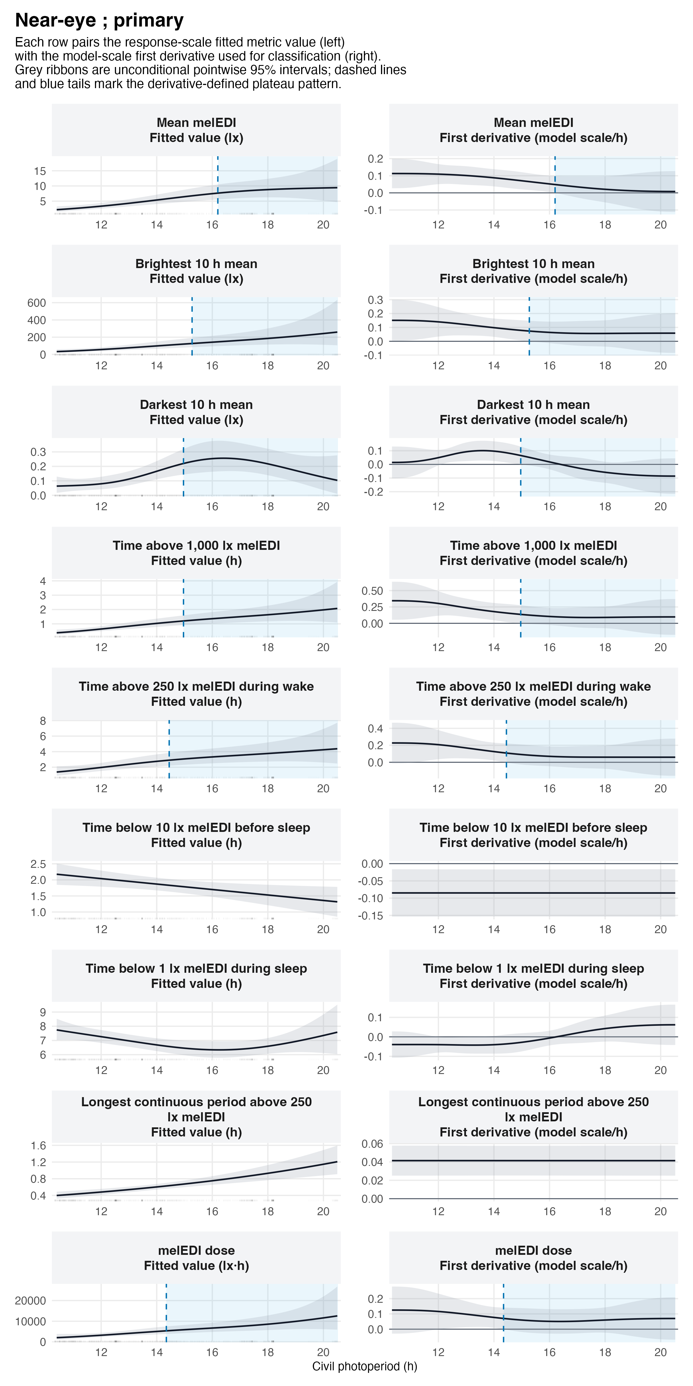
The fitted smooths answer whether an association is visible in the pooled data; the derivative panels apply the stated pattern rule. The figures do not require every site to cover every photoperiod, but the rugs make the uneven empirical support visible.
result_table("near_eye")| Qualifying transition | Qualifying transition bracket (h) | Endpoint derivative | Interpretation | |
|---|---|---|---|---|
| Light level | ||||
| Mean melEDI | Yes | 16.10–16.20 | 0.008 (95% CI -0.111 to 0.127) | Detected increase followed by a sustained zero-compatible tail |
| Brightest 10 h mean | Yes | 15.17–15.27 | 0.059 (95% CI -0.083 to 0.201) | Detected increase followed by a sustained zero-compatible tail |
| Darkest 10 h mean | Yes | 14.86–14.96 | -0.086 (95% CI -0.216 to 0.044) | Detected increase followed by a sustained zero-compatible tail |
| Duration and continuous period | ||||
| Time above 1,000 lx melEDI | Yes | 14.86–14.96 | 0.098 (95% CI -0.176 to 0.371) | Detected increase followed by a sustained zero-compatible tail |
| Time above 250 lx melEDI during wake | Yes | 14.35–14.45 | 0.060 (95% CI -0.159 to 0.279) | Detected increase followed by a sustained zero-compatible tail |
| Time below 10 lx melEDI before sleep | No | ; | -0.085 (95% CI -0.154 to -0.016) | No preceding detected increase |
| Time below 1 lx melEDI during sleep | No | ; | 0.062 (95% CI -0.042 to 0.165) | No preceding detected increase |
| Longest continuous period above 250 lx melEDI | No | ; | 0.041 (95% CI 0.025 to 0.058) | Increase remained detected at the recorded maximum |
| Exposure history | ||||
| melEDI dose | Yes | 14.24–14.35 | 0.070 (95% CI -0.069 to 0.209) | Detected increase followed by a sustained zero-compatible tail |
| A ‘Yes’ is the formal derivative-defined classification: the immediately preceding point has an interval wholly above zero, the next contains zero, and every later interval through the recorded maximum remains zero-compatible. Endpoint derivatives and 95% confidence intervals are on each model’s linear-predictor scale, in model-scale units per hour of civil photoperiod. | ||||
The endpoint derivative for the longest continuous period above 250 lx melEDI remained positive, so this metric did not satisfy the pattern rule. Neither low-light duration had a preceding interval with a pointwise detected positive derivative. For time below 10 lx melEDI before sleep, the endpoint derivative was negative rather than zero-compatible; this is not a positive-to-flat pattern.
The plotted response-scale smooths and derivative calculations are available as smooth source data, derivative source data, and figure settings.
Complementary chest evidence
Depending on the metric, the chest models used 153–154 participants, 743–902 participant-days and observations, and eight sites. The modelled civil-photoperiod range was again 10.33–20.52 h. Tübingen (DE) contributed near-eye but not chest data, which is one reason the chest result is complementary rather than a direct replication on an identical sample.
sample_table("chest")| Participants | Participant-days | Observations | Sites | Civil photoperiod (h) | |
|---|---|---|---|---|---|
| Light level | |||||
| Mean melEDI | 154 | 902 | 902 | 8 | 10.33–20.52 |
| Brightest 10 h mean | 154 | 902 | 902 | 8 | 10.33–20.52 |
| Darkest 10 h mean | 154 | 902 | 902 | 8 | 10.33–20.52 |
| Duration and continuous period | |||||
| Time above 1,000 lx melEDI | 154 | 902 | 902 | 8 | 10.33–20.52 |
| Time above 250 lx melEDI during wake | 154 | 818 | 818 | 8 | 10.33–20.52 |
| Time below 10 lx melEDI before sleep | 153 | 743 | 743 | 8 | 10.33–20.52 |
| Time below 1 lx melEDI during sleep | 154 | 861 | 861 | 8 | 10.33–20.52 |
| Longest continuous period above 250 lx melEDI | 154 | 902 | 902 | 8 | 10.33–20.52 |
| Exposure history | |||||
| melEDI dose | 154 | 851 | 851 | 8 | 10.33–20.52 |
include_project_graphics(file.path(
  root,
  figure_dir,
  "H07_smooth_derivative_pairs_chest.png"
))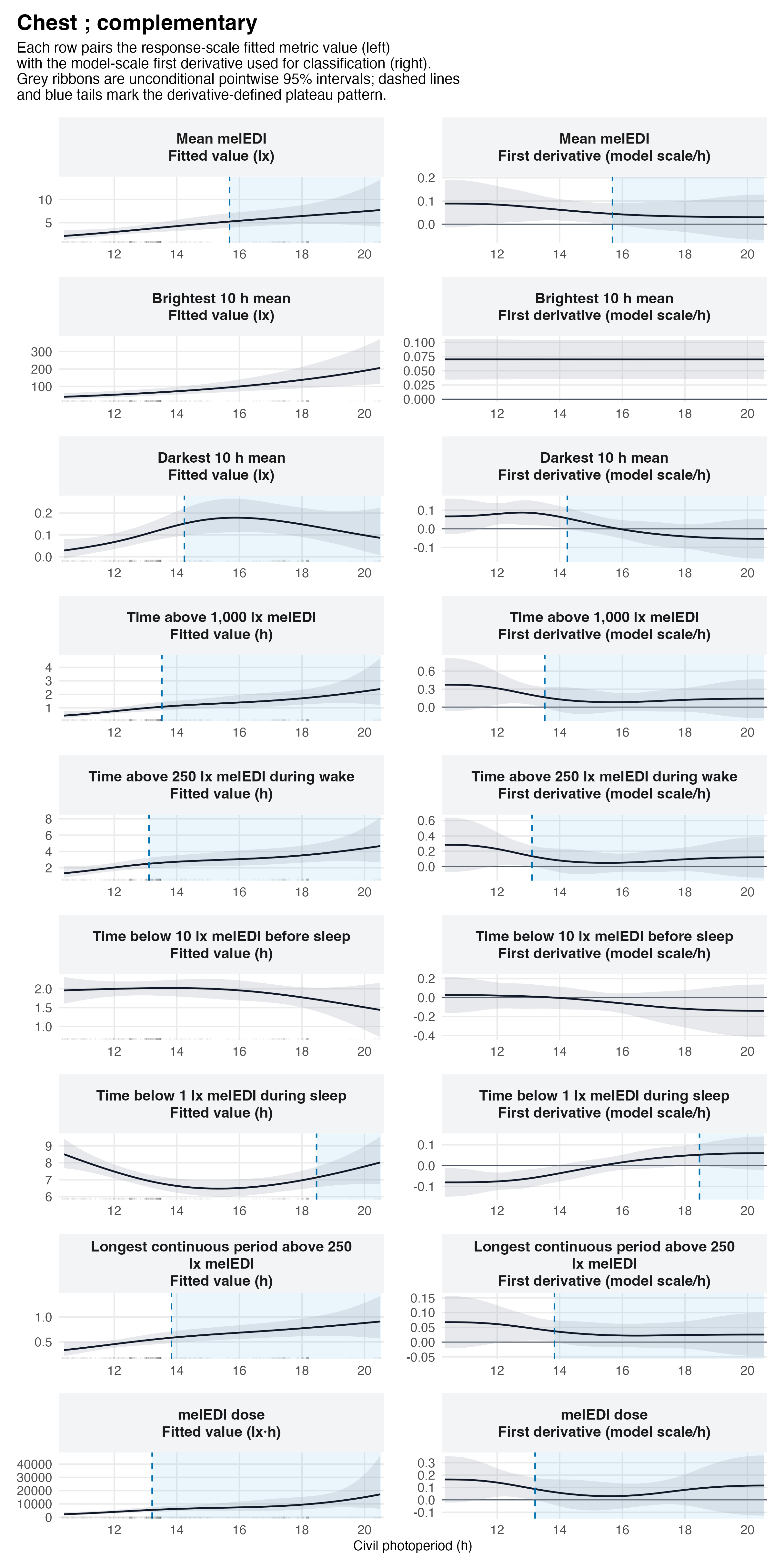
result_table("chest")| Qualifying transition | Qualifying transition bracket (h) | Endpoint derivative | Interpretation | |
|---|---|---|---|---|
| Light level | ||||
| Mean melEDI | Yes | 15.58–15.68 | 0.030 (95% CI -0.067 to 0.128) | Detected increase followed by a sustained zero-compatible tail |
| Brightest 10 h mean | No | ; | 0.070 (95% CI 0.035 to 0.105) | Increase remained detected at the recorded maximum |
| Darkest 10 h mean | Yes | 14.14–14.24 | -0.054 (95% CI -0.161 to 0.053) | Detected increase followed by a sustained zero-compatible tail |
| Duration and continuous period | ||||
| Time above 1,000 lx melEDI | Yes | 13.42–13.52 | 0.141 (95% CI -0.185 to 0.468) | Detected increase followed by a sustained zero-compatible tail |
| Time above 250 lx melEDI during wake | Yes | 13.01–13.11 | 0.120 (95% CI -0.145 to 0.386) | Detected increase followed by a sustained zero-compatible tail |
| Time below 10 lx melEDI before sleep | No | ; | -0.140 (95% CI -0.417 to 0.138) | No preceding detected increase |
| Time below 1 lx melEDI during sleep | Yes | 18.36–18.47 | 0.060 (95% CI -0.020 to 0.140) | Detected increase followed by a sustained zero-compatible tail |
| Longest continuous period above 250 lx melEDI | Yes | 13.73–13.83 | 0.026 (95% CI -0.047 to 0.099) | Detected increase followed by a sustained zero-compatible tail |
| Exposure history | ||||
| melEDI dose | Yes | 13.11–13.21 | 0.116 (95% CI -0.127 to 0.358) | Detected increase followed by a sustained zero-compatible tail |
| A ‘Yes’ is the formal derivative-defined classification: the immediately preceding point has an interval wholly above zero, the next contains zero, and every later interval through the recorded maximum remains zero-compatible. Endpoint derivatives and 95% confidence intervals are on each model’s linear-predictor scale, in model-scale units per hour of civil photoperiod. | ||||
Brightest 10 h mean remained pointwise increasing at the recorded maximum. Time below 10 lx melEDI before sleep again lacked a preceding pointwise detected increase. The late transition for time below 1 lx melEDI during sleep is especially uncertain because its response-distribution check failed, as described below.
Model checks
All 18 reported models converged. Gradients were small and all reported Hessian minima were positive. Residual autocorrelation means that observations close in sequence retain more similar residuals than observations farther apart. Consecutive-day residual autocorrelation was modest in the pooled descriptive check, with maximum absolute lag-1 correlations of 0.229 near eye and 0.154 at the chest. This does not prove temporal independence, but it did not indicate a strong residual day-to-day process after participant clustering.
diagnostic_summary |>
  select(
    "Placement",
    "Converged",
    "Maximum absolute gradient",
    "Minimum Hessian eigenvalue",
    "Basis-check flags",
    "Maximum absolute lag-1",
    "Target/participant concurvity",
    "Deviance explained",
    "Normal-reference QQ correlation"
  ) |>
  gt::gt(rowname_col = "Placement") |>
  gt::fmt_number(
    columns = c(
      `Maximum absolute gradient`,
      `Maximum absolute lag-1`
    ),
    decimals = 4
  ) |>
  gt::fmt_number(
    columns = `Minimum Hessian eigenvalue`,
    decimals = 5
  ) |>
  gt::fmt_integer(columns = `Basis-check flags`) |>
  gt::cols_label(
    `Basis-check flags` = gt::html("Basis flags<br><small>of 9</small>"),
    `Maximum absolute lag-1` = gt::html("Maximum |lag 1|"),
    `Target/participant concurvity` = gt::html(
      "Photoperiod/participant<br>concurvity"
    ),
    `Normal-reference QQ correlation` = gt::html(
      "QQ correlation<br>range"
    )
  ) |>
  gt::cols_width(
    Converged ~ gt::pct(10),
    `Basis-check flags` ~ gt::pct(10),
    `Target/participant concurvity` ~ gt::pct(18),
    `Deviance explained` ~ gt::pct(14),
    `Normal-reference QQ correlation` ~ gt::pct(16)
  ) |>
h07_gt(12)| Converged | Maximum absolute gradient | Minimum Hessian eigenvalue | Basis flags of 9 |
Maximum |lag 1| | Photoperiod/participant concurvity |
Deviance explained | QQ correlation range |
|
|---|---|---|---|---|---|---|---|---|
| Near eye ; primary | 9/9 | 0.0014 | 0.00002 | 2 | 0.2287 | 0.9986–0.9988 | 40.7%–65.6% | 0.952–0.998 |
| Chest ; complementary | 9/9 | 0.0009 | 0.00020 | 1 | 0.1542 | 0.9985–0.9987 | 33.6%–57.6% | 0.960–0.996 |
The basis-dimension check flagged 2 of nine near-eye smooths and 1 of nine chest smooths. These permutation p-values are Monte Carlo diagnostics; their fixed seed makes the reported checks reproducible. The expanded-basis sensitivity therefore carries more weight than a single diagnostic threshold: it reproduced 16 of 17 evaluable classifications, with one near-eye fit failing its Hessian check and the chest sleep low-light classification changing.
Residual normal-reference correlations were generally high, but residuals still showed fitted-value dependence and tail departures for some outcomes. The Tweedie response checks were adequate for the two above-threshold duration metrics. They were not adequate for time below 1 lx melEDI during sleep: each placement had four observed zeros, the fitted model expected fewer than 0.0001 zeros, and none of 100 diagnostic simulations contained a zero. This distributional mismatch makes the chest sleep low-light pattern particularly weak evidence; no larger simulation can repair the response model’s failure to reproduce the observed zero mass.
The photoperiod smooth also had estimated overlap with the participant random-effect smooth (concurvity) of approximately 0.9985–0.9988. This reflects the clustered, repeated-day design and makes their separate contributions harder to distinguish. It limits separation of between-person photoperiod coverage from the pooled smooth. Smooth-term p-values are therefore not used or displayed. The derivative intervals remain conditional on the fitted model and should be read with this identifiability limitation.
Sensitivity analyses
Each sensitivity changed a named feature. The gap-timing-unaware dataset omitted the additional metric-specific adjustment based on when remaining gaps occurred while retaining the coverage rules. The paired/common analysis used only participant-days available at both sensor positions. The cross-dataset common-row analyses restricted the primary and gap-timing-unaware definitions to identical rows. The longest-period analysis retained only days with an exactly identified period, and the dose analysis compared observed and corrected melEDI dose on identical rows. Model-form sensitivities increased photoperiod-smooth flexibility from k = 6 to k = 10 or represented site with fixed rather than random effects. Leave-one-site-out analyses omitted one named site at a time. Agreement below concerns the yes/no qualifying-transition classification, not an identical transition point.
The gap-timing-unaware dataset reproduced all nine near-eye classifications and eight of nine chest classifications; the chest melEDI-dose pattern was the exception. The paired common sample used 110–112 participants, 505–643 participant-days and observations, and eight sites. It reproduced four of nine near-eye and six of nine chest classifications, showing that several pooled patterns depend on which participant-days and sites contribute rather than on placement alone.
sensitivity_sample_summary |>
  select(
    "Scenario",
    "Placement",
    "Participants",
    "Participant-days",
    "Observations",
    "Sites"
  ) |>
  gt::gt(groupname_col = "Scenario") |>
  gt::cols_width(
    Placement ~ gt::pct(16),
    Participants ~ gt::pct(18),
    `Participant-days` ~ gt::pct(21),
    Observations ~ gt::pct(18),
    Sites ~ gt::pct(10)
  ) |>
  gt::tab_source_note(
    gt::md(
      paste0(
        "Preparation exact-common samples were identical for the primary ",
        "and gap-timing-unaware datasets. Observed and corrected dose ",
        "definitions used the same common rows."
      )
    )
  ) |>
h07_gt(12)| Placement | Participants | Participant-days | Observations | Sites |
|---|---|---|---|---|
| Gap-timing-unaware dataset | ||||
| Near eye | 140–141 | 755–811 | 755–811 | 9 |
| Chest | 153–154 | 839–897 | 839–897 | 8 |
| Paired near-eye/chest common sample | ||||
| Near eye | 110–112 | 505–643 | 505–643 | 8 |
| Chest | 110–112 | 505–643 | 505–643 | 8 |
| Preparation exact-common rows | ||||
| Near eye | 139–141 | 653–809 | 653–809 | 9 |
| Chest | 153–154 | 740–894 | 740–894 | 8 |
| Exactly identified longest-period rows | ||||
| Near eye | 132 | 500 | 500 | 9 |
| Chest | 150 | 564 | 564 | 8 |
| Observed/corrected dose common rows | ||||
| Near eye | 141 | 761 | 761 | 9 |
| Chest | 154 | 851 | 851 | 8 |
| Preparation exact-common samples were identical for the primary and gap-timing-unaware datasets. Observed and corrected dose definitions used the same common rows. | ||||
sensitivity_summary |>
  select(
    "Scenario",
    "Placement",
    "Agreement",
    "Changed classifications"
  ) |>
  gt::gt(groupname_col = "Scenario") |>
  gt::cols_width(
    Placement ~ gt::pct(14),
    Agreement ~ gt::pct(12),
    `Changed classifications` ~ gt::pct(56)
  ) |>
  gt::tab_source_note(
    gt::md(
      paste0(
        "Agreement concerns the yes/no qualifying-transition classification only; transition ",
        "brackets can move even when the classification agrees."
      )
    )
  ) |>
h07_gt(12)| Placement | Agreement | Changed classifications |
|---|---|---|
| Gap-timing-unaware dataset | ||
| Near eye ; primary | 9/9 | None |
| Chest ; complementary | 8/9 | melEDI dose |
| Paired near-eye/chest common sample | ||
| Near eye ; primary | 4/9 | Brightest 10 h mean; Darkest 10 h mean; Time above 1,000 lx melEDI; Time above 250 lx melEDI during wake; melEDI dose |
| Chest ; complementary | 6/9 | Time below 1 lx melEDI during sleep; Longest continuous period above 250 lx melEDI; melEDI dose |
| Preparation exact-common rows: primary dataset | ||
| Near eye ; primary | 9/9 | None |
| Chest ; complementary | 8/9 | Time below 1 lx melEDI during sleep |
| Preparation exact-common rows: gap-timing-unaware dataset | ||
| Near eye ; primary | 9/9 | None |
| Chest ; complementary | 8/9 | Time below 1 lx melEDI during sleep |
| Exactly identified longest-period rows | ||
| Near eye ; primary | 0/1 | Longest continuous period above 250 lx melEDI |
| Chest ; complementary | 1/1 | None |
| Observed/corrected dose on common rows | ||
| Near eye ; primary | 2/2 | None |
| Chest ; complementary | 2/2 | None |
| Agreement concerns the yes/no qualifying-transition classification only; transition brackets can move even when the classification agrees. | ||
Restricting the longest continuous period above 250 lx melEDI to days whose period duration was exactly identified changed the near-eye classification from no pattern to a pattern at 15.38–15.48 h; the chest classification was unchanged. Comparing the observed and corrected melEDI-dose definitions on identical rows left both placement classifications unchanged. Restricting the two preparation variants to exact common rows preserved every near-eye classification but removed the chest sleep low-light pattern in both variants.
model_form_summary |>
  select(
    "Model",
    "Placement",
    "Agreement",
    "Failed fits",
    "Changed classifications"
  ) |>
  gt::gt(groupname_col = "Model") |>
  gt::fmt_integer(columns = `Failed fits`) |>
  gt::cols_width(
    Placement ~ gt::pct(14),
    Agreement ~ gt::pct(12),
    `Failed fits` ~ gt::pct(12),
    `Changed classifications` ~ gt::pct(48)
  ) |>
h07_gt(12)| Placement | Agreement | Failed fits | Changed classifications |
|---|---|---|---|
| Expanded smooth basis (k = 10) | |||
| Near eye ; primary | 8/8 | 1 | None |
| Chest ; complementary | 8/9 | 0 | Time below 1 lx melEDI during sleep |
| Site as a fixed effect | |||
| Near eye ; primary | 8/9 | 0 | Longest continuous period above 250 lx melEDI |
| Chest ; complementary | 8/9 | 0 | Time below 1 lx melEDI during sleep |
The broader smooth reproduced eight of eight evaluable near-eye and eight of nine chest classifications; the near-eye longest-period fit failed its Hessian check, and the chest sleep low-light pattern disappeared. Treating site as a fixed effect reproduced eight of nine classifications at each placement: the near-eye longest-period pattern appeared, while the chest sleep low-light pattern disappeared. These changes reinforce that both metrics sit near a classification boundary.
Site influence and support
Omitting one site at a time did not act as a new eligibility rule; it tested whether a pooled pattern depended strongly on one site’s observations. Near-eye mean melEDI and both low-light metrics reproduced their main classification in all nine omissions. Five positive near-eye patterns changed only when Tübingen (DE) was omitted. The near-eye longest-period classification changed in four of nine omissions. Chest results were less stable for several outcomes, most notably time below 1 lx melEDI during sleep, which matched the main classification in only three of eight omissions.
loso_table("near_eye")| Matching omissions | Discordant site omissions | Transition range when present (h) | |
|---|---|---|---|
| Light level | |||
| Mean melEDI | 9/9 | None | 15.38–16.41 |
| Brightest 10 h mean | 8/9 | Tübingen (DE) | 13.83–16.41 |
| Darkest 10 h mean | 8/9 | Tübingen (DE) | 14.24–15.07 |
| Duration and continuous period | |||
| Time above 1,000 lx melEDI | 8/9 | Tübingen (DE) | 13.44–16.51 |
| Time above 250 lx melEDI during wake | 8/9 | Tübingen (DE) | 13.68–14.86 |
| Time below 10 lx melEDI before sleep | 9/9 | None | ; |
| Time below 1 lx melEDI during sleep | 9/9 | None | ; |
| Longest continuous period above 250 lx melEDI | 5/9 | Dortmund (DE); Madrid (ES); San José (CR); Kumasi (GH) | 15.05–16.20 |
| Exposure history | |||
| melEDI dose | 8/9 | Tübingen (DE) | 13.76–15.99 |
loso_table("chest")| Matching omissions | Discordant site omissions | Transition range when present (h) | |
|---|---|---|---|
| Light level | |||
| Mean melEDI | 8/8 | None | 13.76–16.10 |
| Brightest 10 h mean | 6/8 | Izmir (TR); Kumasi (GH) | 12.70–15.07 |
| Darkest 10 h mean | 7/8 | Izmir (TR) | 13.36–14.45 |
| Duration and continuous period | |||
| Time above 1,000 lx melEDI | 8/8 | None | 12.48–14.45 |
| Time above 250 lx melEDI during wake | 6/8 | Delft (NL); Izmir (TR) | 12.16–13.52 |
| Time below 10 lx melEDI before sleep | 8/8 | None | ; |
| Time below 1 lx melEDI during sleep | 3/8 | Borås (SE); Munich (DE); Madrid (ES); Izmir (TR); San José (CR) | 18.47–18.67 |
| Longest continuous period above 250 lx melEDI | 7/8 | Borås (SE) | 13.13–15.48 |
| Exposure history | |||
| melEDI dose | 7/8 | Izmir (TR) | 12.80–14.35 |
The observed civil-photoperiod range was broad overall but uneven across sites. For example, near-eye observations ranged from 10.33 to 12.35 h in Madrid (ES), 16.41 to 17.45 h in Munich (DE), and 12.49 to 12.71 h in Kumasi (GH); San José (CR) contributed only a narrow range around 13.47 h, while Borås (SE) covered values up to 20.52 h. Sites were also measured in different collection periods and, in some cases, different years. Thus the pooled smooth can answer whether an association is visible in this dataset, but it cannot separate photoperiod from every site-specific or collection-period difference. Leave-one-site-out changes show where this limitation affects the descriptive classification.
Interpretation and limitations
The pooled analysis shows several fitted photoperiod associations that rise and then meet the prespecified pointwise rule for a sustained zero-compatible derivative. The recurring patterns for mean melEDI, darkest 10 h mean, both above-threshold duration metrics, and melEDI dose across the two placements are the most consistent descriptive findings. Brightest 10 h mean differs by placement, the longest-period result is sensitive to sample definition and model form, and the chest sleep low-light result is undermined by distributional failure, common-row analyses, model-form changes, and site influence.
The strongest defensible conclusion is therefore that qualifying transitions from increase to a sustained near-flat tail are visible for several personal light-exposure metrics in the pooled data, subject to substantial design and model limitations. The results do not establish a ceiling, an equivalence region, a causal effect of photoperiod, a distinct latitude effect, a health or clinical consequence, or equivalence between near-eye and chest placement.
Preregistration deviations
- H07 predictors and outcome selection: the registered latitude-by-photoperiod surface is non-identifiable here, so the retained report retains all nine outcomes and presents a separately labelled site-adjusted nonlinear photoperiod analysis as descriptive evidence.
- H07 outcome selection and multiplicity: all nine eligible outcomes remain visible rather than being selected using H01 significance or H07 AIC.
- H07 response model: response specifications and model checks are metric-specific rather than one universal zero-aware log-Gaussian model.
Footnotes
The stored formal method label is derivative-defined plateau pattern. It denotes only the three-part pointwise classification above; it is not a biological-ceiling, permanent-plateau, or equivalence claim.↩︎