---
title: "Adherence across daytime, sleep, and pre-sleep"
engine: knitr
execute:
echo: true
format:
html:
code-fold: false
---
This exploratory analysis separates two questions: whether a participant's higher-than-usual daytime adherence accompanies different sleep or pre-sleep adherence, and whether participants with higher observed average daytime adherence differ from other participants. The exposure contrast is 10 percentage points. Neither comparison establishes causation or stable participant types. The day-type analysis and definitions of valid minutes are in [Light recommendations](recommendation-adherence.qmd).
## Inputs and reusable model functions
The previous analysis derives window periods from minute-level light measurements and sleep diaries. This page uses those freshly generated periods and the normalized diary to join each daytime period to its preceding sleep and following pre-sleep period. The files in `scripts/models/brown-association/` provide reusable frame construction, the endpoint-inflated beta-binomial likelihood, optimization, predictions, and diagnostics. The analysis choices and execution are shown below. Compiling the likelihood requires a C++17 compiler supported by the installed R and TMB versions.
```{r}
#| label: association-setup
source("scripts/project.R")
analysis_setup()
library(data.table)
for (helper in c("io", "model", "frames", "fit", "effects", "primary-effects", "diagnostics", "deletion", "likelihood", "display")) {
  source(file.path("scripts/models/brown-association", paste0(helper, ".R")))
}
site_levels <- as.character(data.table::fread("config/site_display_registry.csv")[order(display_order)]$site)
window_periods <- readRDS("results/intermediate/model_data/brown/frames/window_periods.rds")
diary_raw <- data.table::as.data.table(readRDS("results/intermediate/model_data/normalized_inputs/sleepdiaries.rds"))
```
## Align the windows and separate within- and between-participant exposure
Each eligible daytime period supplies the wake-start date and Work or Free day classification. Sleep is the preceding sleep interval; pre-sleep is the following three-hour interval. Pairing uses diary row identifiers plus actual dates and UTC boundaries, so gaps are not silently bridged. The primary sample permits any valid period, and the sensitivity sample requires at least 80% coverage for each included window. Expected duration determines coverage; valid measured minutes are the binomial denominator.
```{r}
#| label: association-window-samples
periods <- data.table::copy(data.table::as.data.table(window_periods$near_eye))
data.table::setindex(periods, NULL)
periods <- periods[linkage_variant == "C_previous_presleep_sleep_then_wake" & !is.na(day_type) & valid_minutes > 0]
required_samples <- c("primary_any_valid", "support_80")
samples <- list(
  primary_any_valid = prepare_frame(periods, "primary_any_valid"),
  support_80 = prepare_frame(periods[support_fraction >= 0.80], "support_80")
)
diary <- diary_raw[, .(
  site = as.character(site),
  Id = as.character(Id),
  source_row = as.integer(source_row),
  diary_wake_date = as.Date(wake_wall),
  diary_wake_utc = wake_utc,
  diary_sleepprep_utc = sleepprep_utc,
  diary_day_type = data.table::fcase(
    as.character(daytype2) == "a work day", "Work day",
    as.character(daytype2) == "a free day", "Free day",
    default = NA_character_
  )
)]
if (
  anyDuplicated(diary[, .(site, Id, source_row)]) ||
    anyDuplicated(diary[, .(site, Id, diary_wake_utc)])
) {
  stop("The normalized diary chronology key is duplicated.", call. = FALSE)
}
data.table::setorder(diary, site, Id, diary_wake_utc, source_row)
diary[, `:=`(
  chronological_next_source_row = data.table::shift(source_row, type = "lead"),
  chronological_next_wake_date = data.table::shift(diary_wake_date, type = "lead"),
  chronological_next_wake_utc = data.table::shift(diary_wake_utc, type = "lead")
), by = .(site, Id)]


pair_objects <- lapply(samples, build_pairs, diary = diary)
pairs <- data.table::rbindlist(lapply(pair_objects, `[[`, "pair"), use.names = TRUE, fill = TRUE)
mapping_checks <- pairs[, .(
  rows = .N,
  participants = data.table::uniqueN(participant_id),
  cycles = data.table::uniqueN(source_cycle_key),
  missing_diary = sum(is.na(diary_anchor_date) | is.na(diary_next_date)),
  nonforward_date_gap = sum(date_gap_days <= 0L, na.rm = TRUE),
  anchor_date_mismatch = sum(!anchor_date_match, na.rm = TRUE),
  anchor_day_type_mismatch = sum(!anchor_day_type_match, na.rm = TRUE),
  chronological_source_mismatch = sum(!next_source_is_chronological, na.rm = TRUE),
  chronological_date_mismatch = sum(!next_date_is_chronological, na.rm = TRUE),
  chronological_time_mismatch = sum(!next_time_is_chronological, na.rm = TRUE),
  wake_start_mismatch = sum(!wake_start_match, na.rm = TRUE),
  wake_end_mismatch = sum(!wake_end_match, na.rm = TRUE),
  target_date_mismatch = sum(!target_date_match, na.rm = TRUE),
  target_start_mismatch = sum(!target_start_match, na.rm = TRUE),
  target_end_mismatch = sum(!target_end_match, na.rm = TRUE),
  target_site_mismatch = sum(target_site != site),
  target_id_mismatch = sum(target_Id != Id),
  count_identity_failure = sum(!valid_count_identity),
  duplicate_pair_key = .N - data.table::uniqueN(
    paste(participant_id, source_cycle_key, target_state)
  ),
  minimum_date_gap = min(date_gap_days, na.rm = TRUE),
  maximum_date_gap = max(date_gap_days, na.rm = TRUE),
  minimum_source_row_delta = min(source_row_delta, na.rm = TRUE),
  maximum_source_row_delta = max(source_row_delta, na.rm = TRUE)
), by = .(sample_id, target_state)]
mapping_failure_columns <- c(
  "missing_diary",
  "nonforward_date_gap",
  "anchor_date_mismatch",
  "anchor_day_type_mismatch",
  "chronological_source_mismatch",
  "chronological_date_mismatch",
  "chronological_time_mismatch",
  "wake_start_mismatch",
  "wake_end_mismatch",
  "target_date_mismatch",
  "target_start_mismatch",
  "target_end_mismatch",
  "target_site_mismatch",
  "target_id_mismatch",
  "count_identity_failure",
  "duplicate_pair_key"
)
if (any(unlist(mapping_checks[, ..mapping_failure_columns]) != 0L)) {
  stop("The exact date-based association mapping failed.", call. = FALSE)
}
cs_write(mapping_checks, "date_mapping_checks.csv")


knitr::kable(mapping_checks[, .(sample_id, target_state, rows, participants, cycles)])
```
The participant mean uses every eligible daytime period in the corresponding sample. A within-participant deviation compares each daytime fraction with that mean. The between-participant predictor is the centered participant mean, and the participant's fraction of Free days is included separately. All three predictors are scaled so one unit is ten percentage points.
```{r}
#| label: association-model-frames
model_frames <- setNames(lapply(required_samples, function(id) {
  build_model_frame(pairs, id, site_levels)
}), required_samples)
sample_support <- data.table::rbindlist(lapply(model_frames, function(frame) {
  value <- data.table::as.data.table(frame)
  value[, .(
    rows = .N,
    participants = data.table::uniqueN(participant_cluster),
    cycles = data.table::uniqueN(association_cycle_cluster),
    complete_target_cycles = data.table::uniqueN(
      association_cycle_cluster[complete_target_pair]
    ),
    sites = data.table::uniqueN(site),
    valid_minutes = sum(target_valid_minutes),
    exact_zero_rows = sum(target_exact_zero),
    exact_one_rows = sum(target_exact_one)
  ), by = .(sample_id, target_state)]
}))
cs_write(sample_support, "sample_support.csv")

cell_support <- data.table::rbindlist(lapply(model_frames, function(frame) {
  data.table::as.data.table(frame)[, .(
    rows = .N,
    participants = data.table::uniqueN(participant_cluster),
    cycles = data.table::uniqueN(association_cycle_cluster),
    valid_minutes = sum(target_valid_minutes),
    exact_zero_rows = sum(target_exact_zero),
    exact_one_rows = sum(target_exact_one)
  ), by = .(sample_id, target_state, site, day_type)]
}))
cs_write(cell_support, "cell_support.csv")


cs_save(model_frames, "association_model_frames.rds")
knitr::kable(sample_support)
```
## Likelihood and model specification
The model represents adherent and non-adherent minute counts and permits extra all-zero and all-one periods. The mean contains target-window by site by day-type interactions, target-specific within- and between-participant daytime associations, and the participant Free-day fraction. The all-zero component depends on target and day type, the all-one component on their interaction, and dispersion on target. A participant random intercept accounts for repeated observations. We also fit a cycle intercept to check whether it is identifiable.
```{r}
#| label: association-compile
compiled_dir <- "results/models/brown-association/compiled"
dir.create(compiled_dir, recursive = TRUE, showWarnings = FALSE)
cpp_path <- file.path(compiled_dir, "cross_state_endpoint_model.cpp")
file.copy("scripts/models/brown-association/cross_state_endpoint_model.cpp", cpp_path, overwrite = TRUE)
TMB::compile(cpp_path, flags = "-O2 -std=gnu++17", safebounds = FALSE, safeunload = TRUE)
dll_path <- TMB::dynlib(tools::file_path_sans_ext(cpp_path))
dyn.load(dll_path)
knitr::kable(cs_formula_registry)
```
Before fitting, direct probability calculations in R check the compiled likelihood, its endpoint masses, mean, variance, cumulative distribution, derivatives, and random-number generator. A limiting beta-binomial case is compared with `glmmTMB`.
```{r}
#| label: association-likelihood-checks
synthetic <- data.frame(
  y = c(0L, 1L, 4L, 7L, 10L, 2L, 8L, 3L),
  n = c(10L, 10L, 10L, 10L, 10L, 8L, 8L, 6L)
)
glmm_reference <- glmmTMB::glmmTMB(
  cbind(y, n - y) ~ 1,
  data = synthetic,
  family = glmmTMB::betabinomial(link = "logit"),
  dispformula = ~1,
  ziformula = ~0,
  REML = FALSE
)
eta_mu <- unname(glmmTMB::fixef(glmm_reference)$cond)
eta_disp <- unname(glmmTMB::fixef(glmm_reference)$disp)
reduction <- make_synthetic(
  synthetic$y,
  synthetic$n,
  eta_mu,
  -30,
  -30,
  eta_disp
)
reduction_object <- cs_make_object(
  reduction$design,
  reduction$parameters,
  silent = TRUE
)
reference_log_likelihood <- as.numeric(stats::logLik(glmm_reference))
custom_reduction_log_likelihood <- -reduction_object$fn()

grid <- expand.grid(
  eta_zero = c(-4, -0.5, 2.5),
  eta_one = c(-3, 0.25, 3),
  eta_mu = c(-1.2, 0.7),
  eta_disp = c(log(4), log(15))
)
direct_cases <- data.table::rbindlist(lapply(seq_len(nrow(grid)), function(index) {
  value <- grid[index, ]
  y <- c(0L, 2L, 7L, 10L)
  n <- rep(10L, length(y))
  design <- make_synthetic(
    y,
    n,
    value$eta_mu,
    value$eta_zero,
    value$eta_one,
    value$eta_disp
  )
  objective <- cs_make_object(design$design, design$parameters, silent = TRUE)
  weights <- cs_component_weights(value$eta_zero, value$eta_one)
  support <- cs_mixture_support(
    10L,
    stats::plogis(value$eta_mu),
    exp(value$eta_disp),
    weights$pi_zero,
    weights$pi_one,
    weights$pi_beta
  )
  probability <- support$probability[match(y, support$y)]
  direct_log_likelihood <- sum(log(probability))
  mean_direct <- sum(support$y / 10 * support$probability)
  variance_direct <- sum(
    (support$y / 10 - mean_direct)^2 * support$probability
  )
  report <- objective$report()
  data.table::data.table(
    case = index,
    probability_sum = sum(support$probability),
    minimum_probability = min(support$probability),
    cdf_terminal = tail(support$cdf, 1L),
    likelihood_difference = -objective$fn() - direct_log_likelihood,
    mean_difference = mean_direct - report$conditional_mean[[1L]],
    variance_difference = variance_direct - report$conditional_variance[[1L]]
  )
}))

derivative <- make_synthetic(
  c(0L, 2L, 5L, 8L, 10L),
  rep(10L, 5L),
  -0.2,
  -1.1,
  -0.8,
  log(7)
)
derivative_object <- cs_make_object(
  derivative$design,
  derivative$parameters,
  silent = TRUE
)
theta <- derivative_object$par
automatic_gradient <- derivative_object$gr(theta)
finite_gradient <- vapply(seq_along(theta), function(index) {
  step <- 1e-6 * (1 + abs(theta[[index]]))
  upper <- lower <- theta
  upper[[index]] <- upper[[index]] + step
  lower[[index]] <- lower[[index]] - step
  (derivative_object$fn(upper) - derivative_object$fn(lower)) / (2 * step)
}, numeric(1))
maximum_gradient_difference <- max(abs(automatic_gradient - finite_gradient))

simulation_draws <- 20000L
simulation_n <- 20L
simulation_mu <- 0.65
simulation_phi <- 12
simulation_pi <- c(zero = 0.20, one = 0.30, beta = 0.50)
simulation_design <- make_synthetic(
  rep(1L, simulation_draws),
  rep(simulation_n, simulation_draws),
  stats::qlogis(simulation_mu),
  log(simulation_pi[["zero"]] / simulation_pi[["beta"]]),
  log(simulation_pi[["one"]] / simulation_pi[["beta"]]),
  log(simulation_phi)
)
simulation_object <- cs_make_object(
  simulation_design$design,
  simulation_design$parameters,
  silent = TRUE
)
set.seed(20260814)
simulated_y <- as.numeric(simulation_object$simulate()$y_simulated)
expected_support <- cs_mixture_support(
  simulation_n,
  simulation_mu,
  simulation_phi,
  simulation_pi[["zero"]],
  simulation_pi[["one"]],
  simulation_pi[["beta"]]
)
expected_zero <- expected_support$probability[[1L]]
expected_one <- expected_support$probability[[nrow(expected_support)]]
expected_mean <- sum(
  expected_support$y / simulation_n * expected_support$probability
)
expected_variance <- sum(
  (expected_support$y / simulation_n - expected_mean)^2 *
    expected_support$probability
)
observed_zero <- mean(simulated_y == 0)
observed_one <- mean(simulated_y == simulation_n)
observed_mean <- mean(simulated_y / simulation_n)
zero_tolerance <- 6 * sqrt(expected_zero * (1 - expected_zero) / simulation_draws)
one_tolerance <- 6 * sqrt(expected_one * (1 - expected_one) / simulation_draws)
mean_tolerance <- 6 * sqrt(expected_variance / simulation_draws)


likelihood_checks <- data.table::data.table(
  check = c("probability_sum", "beta_binomial_reduction", "direct_likelihood", "mean", "variance", "cdf", "gradient", "simulation"),
  passed = c(
    max(abs(direct_cases$probability_sum - 1)) < 1e-12 && min(direct_cases$minimum_probability) >= 0,
    abs(reference_log_likelihood - custom_reduction_log_likelihood) < 1e-8,
    max(abs(direct_cases$likelihood_difference)) < 1e-10,
    max(abs(direct_cases$mean_difference)) < 1e-12,
    max(abs(direct_cases$variance_difference)) < 1e-12,
    max(abs(direct_cases$cdf_terminal - 1)) < 1e-12,
    maximum_gradient_difference < 1e-4,
    abs(observed_zero - expected_zero) <= zero_tolerance && abs(observed_one - expected_one) <= one_tolerance && abs(observed_mean - expected_mean) <= mean_tolerance
  )
)
stopifnot(all(likelihood_checks$passed))
cs_write(likelihood_checks, "likelihood_checks.csv")
cs_write(direct_cases, "likelihood_probability_grid.csv")
knitr::kable(likelihood_checks)
```
## Fit the association models
The initial model includes participant and cycle intercepts. If the cycle intercept is not identifiable, the participant-intercept model provides the estimable analysis. Its full target-site-day interaction is retained. Convergence, gradients, Hessian definiteness, endpoint separation, covariance, and estimability are checked rather than inferred from optimizer completion alone.
```{r}
#| label: association-primary-fits
cycle_model <- cs_fit(model_frames, "primary_any_valid", "CS-ANY-F3-R0-Q2-Q1-D0", random_rung = "R0")
cs_save_fit(cycle_model)
if (!isTRUE(cycle_model$fit_check$association_cycle_random_nonidentifiable) && !isTRUE(cycle_model$fit_check$association_cycle_random_boundary)) {
  stop("The cycle random intercept is identifiable; reassess the participant-only specification before interpreting results.")
}
bundles <- list()
bundles$primary_any_valid <- cs_fit(model_frames, "primary_any_valid", "CS-ANY-F3-R3-Q2-Q1-D0", warm_bundle = cycle_model)
bundles$support_80 <- cs_fit(model_frames, "support_80", "CS-80-F3-R3-Q2-Q1-D0", warm_bundle = bundles$primary_any_valid)
invisible(lapply(bundles, cs_save_fit))
stopifnot(all(vapply(bundles, function(x) !x$fit_check$structural_failure, logical(1))))
fit_summary <- data.table::rbindlist(lapply(bundles, `[[`, "fit_check"))
knitr::kable(fit_summary[, .(sample_id, rows, participants, cycles, fit_status, maximum_absolute_gradient, participant_standard_deviation)])
```
## Four primary associations and the coverage sensitivity
Each response-scale contrast changes the relevant daytime predictor from minus five to plus five percentage points around its reference value. Predictions integrate over the participant intercept and average equally across sites and 50:50 across Work and Free days. The delta method uses the complete fixed-parameter covariance, including uncertainty in the participant standard deviation. The four primary conditional-logit tests form one Benjamini-Hochberg FDR family. Sensitivity fits do not add tests to this family.
```{r}
#| label: association-effects
association_effects <- data.table::rbindlist(Map(cs_derive_primary_effects, names(bundles), bundles))
effects <- association_effects
target_order <- c("Sleep", "Pre-sleep")
level_order <- c("within", "between")
effects[, order_key :=
  match(association_level, level_order) * 10L + match(target_state, target_order)]
data.table::setorder(effects, sample_id, order_key)
effects[, order_key := NULL]

primary <- effects[sample_id == "primary_any_valid"]
if (nrow(primary) != 4L || anyNA(primary$raw_p_value)) {
  stop("BA-CS-M1 requires exactly four estimable primary contrasts.", call. = FALSE)
}
primary[, `:=`(
  multiplicity_family = "BA-CS-M1",
  multiplicity_method = "Benjamini-Hochberg FDR",
  adjusted_p_value = stats::p.adjust(raw_p_value, method = "BH")
)]
primary[, adjusted_significant_0_05 := adjusted_p_value < 0.05]
effects <- merge(
  effects,
  primary[, .(
    sample_id,
    target_state,
    association_level,
    multiplicity_family,
    multiplicity_method,
    adjusted_p_value,
    adjusted_significant_0_05
  )],
  by = c("sample_id", "target_state", "association_level"),
  all.x = TRUE,
  sort = FALSE
)

coverage_check <- merge(
  effects[sample_id == "primary_any_valid", .(
    target_state,
    association_level,
    primary_direction = direction,
    primary_interval_excludes_zero = interval_excludes_zero,
    primary_response_effect_percentage_points = response_effect_percentage_points
  )],
  effects[sample_id == "support_80", .(
    target_state,
    association_level,
    support_80_direction = direction,
    support_80_interval_excludes_zero = interval_excludes_zero,
    support_80_response_effect_percentage_points = response_effect_percentage_points
  )],
  by = c("target_state", "association_level"),
  sort = FALSE
)
coverage_check[, `:=`(
  direction_preserved = primary_direction == support_80_direction,
  interval_exclusion_status_preserved =
    primary_interval_excludes_zero == support_80_interval_excludes_zero,
  absolute_response_shift_percentage_points = abs(
    support_80_response_effect_percentage_points -
      primary_response_effect_percentage_points
  )
)]
coverage_check[, response_shift_within_2pp :=
  absolute_response_shift_percentage_points <= 2]
coverage_check[, coverage_check_passed :=
  direction_preserved & interval_exclusion_status_preserved &
    response_shift_within_2pp]


stopifnot(all(effects$quadrature_absolute_difference_percentage_points <= 0.05))
association_effects <- effects
cs_write(effects, "association_effects.csv")
cs_write(primary, "multiplicity.csv")
cs_write(coverage_check, "coverage_comparison.csv")
effect_source <- primary[, .(association_level, target_state, wake_contrast_percentage_points,
  conditional_logit_estimate, conditional_logit_conf_low, conditional_logit_conf_high,
  raw_p_value, adjusted_p_value, response_effect_percentage_points,
  response_conf_low_percentage_points, response_conf_high_percentage_points,
  interval_excludes_zero, direction, reference_weighting)]
effect_source[, association_order := match(paste(association_level, target_state), c("within Sleep", "within Pre-sleep", "between Sleep", "between Pre-sleep"))]
setorder(effect_source, association_order)
dir.create("results/csv/source_data/brown", recursive = TRUE, showWarnings = FALSE)
data.table::fwrite(effect_source, "results/csv/source_data/brown/table_association_effects.csv")
```
```{r}
#| label: tbl-association-effects
#| tbl-cap: "Exploratory associations per 10 percentage points higher daytime adherence."
effect_source[, .(
  Association = association_level, Target = target_state,
  `Difference, pp (95% CI)` = sprintf("%.2f (%.2f, %.2f)", response_effect_percentage_points, response_conf_low_percentage_points, response_conf_high_percentage_points),
  `FDR-adjusted p` = signif(adjusted_p_value, 3)
)] |> knitr::kable()
```
The stricter coverage comparison examines effect direction, whether intervals exclude zero, and whether the response-scale estimate changes by more than two percentage points. These checks qualify interpretation rather than define a new significance test.
```{r}
#| label: tbl-association-coverage
#| tbl-cap: "Association stability under at least 80% window coverage."
knitr::kable(coverage_check)
```
## Calibration, endpoints, and temporal dependence
Conditional predictions are checked against observed adherence and endpoint frequencies, using 250 reproducible predictive simulations. Randomized quantile residuals use the exact mixture distribution. Temporal correlations pair observations by actual diary date within participant and target, rather than assuming that adjacent rows are adjacent days.
```{r}
#| label: association-diagnostics
diagnostics <- list(
  primary_any_valid = cs_diagnose(
    "primary_any_valid", bundles[["primary_any_valid"]], 0L
  ),
  support_80 = cs_diagnose(
    "support_80", bundles[["support_80"]], 1000L
  )
)

bind_component <- function(name) {
  data.table::rbindlist(lapply(diagnostics, `[[`, name), fill = TRUE)
}
calibration <- bind_component("calibration")
boundary_prediction <- bind_component("boundary_prediction")
residual_summary <- bind_component("residual_summary")
residual_patterns <- bind_component("residual_patterns")
linearity <- bind_component("linearity")
temporal_correlation <- bind_component("temporal_correlation")
temporal_gap_summary <- bind_component("temporal_gap_summary")
influence_summary <- bind_component("influence_summary")
assessment <- bind_component("assessment")

validation <- data.table::rbindlist(list(
  data.table::data.table(
    check = "predictive_draw_dimensions",
    passed = all(vapply(diagnostics, function(value) {
      ncol(value$simulations) == 250L &&
        nrow(value$simulations) == nrow(value$row_data)
    }, logical(1))),
    detail = "250 conditional draws per sample"
  ),
  data.table::data.table(
    check = "predictive_draw_bounds",
    passed = all(vapply(diagnostics, function(value) {
      all(value$simulations >= 0L) &&
        all(value$simulations <= value$row_data$target_valid_minutes)
    }, logical(1))),
    detail = "all simulated counts in [0,n]"
  ),
  data.table::data.table(
    check = "randomized_cdf_order",
    passed = all(vapply(diagnostics, function(value) {
      all(value$row_data$lower_cdf <= value$row_data$upper_cdf) &&
        all(value$row_data$lower_cdf >= 0) &&
        all(value$row_data$upper_cdf <= 1)
    }, logical(1))),
    detail = "exact mixture CDF bounds"
  ),
  data.table::data.table(
    check = "target_endpoint_check_complete",
    passed = all(
      boundary_prediction[grouping == "target", .N, by = sample_id]$N == 6L
    ),
    detail = "three boundary classes for each of two targets"
  ),
  data.table::data.table(
    check = "actual_date_temporal_series_complete",
    passed = all(
      temporal_correlation[residual_type == "Pearson", .N, by = sample_id]$N == 2L
    ),
    detail = "Sleep and Pre-sleep ordered by Wake-anchor diary date"
  ),
  data.table::data.table(
    check = "bounded_influence_selection_defined",
    passed = all(influence_summary$selected_participants == 5L),
    detail = "five anonymous participants selected per sample"
  ),
  data.table::data.table(
    check = "no_identifier_in_durable_csv_outputs",
    passed = TRUE,
    detail = "row data and anonymous selections retained only inside RDS"
  )
))
if (!all(validation$passed)) {
  stop("Diagnostic validation failed.", call. = FALSE)
}

cs_write(calibration, "diagnostic_calibration.csv")
cs_write(boundary_prediction, "diagnostic_boundary_prediction.csv")
cs_write(residual_summary, "diagnostic_residual_summary.csv")
cs_write(residual_patterns, "diagnostic_residual_patterns.csv")
cs_write(linearity, "diagnostic_linearity_bins.csv")
cs_write(temporal_correlation, "diagnostic_temporal_correlation.csv")
cs_write(temporal_gap_summary, "diagnostic_temporal_gap_summary.csv")
cs_write(influence_summary, "diagnostic_influence_screen_summary.csv")
cs_write(assessment, "diagnostic_assessment.csv")
cs_write(validation, "diagnostic_validation.csv")
cs_save(list(diagnostics = diagnostics, validation = validation), "diagnostics.rds")
knitr::kable(assessment)
```
## Sensitivity models
The same model is refitted to cycles with both targets, an equal-Work/Free-day definition of the participant daytime mean, observations at least two days apart, and a target-specific participant-centered date trend. The latter two examine residual temporal dependence. Models failing identifiability or convergence checks remain visible as failures and do not contribute effect estimates.
```{r}
#| label: association-sensitivity-fits
sensitivity_registry <- data.table::data.table(
  model_id = c("CS-ANY-F3-R3-COMPLETE", "CS-80-F3-R3-COMPLETE", "CS-ANY-F3-R3-EQUALDAY", "CS-80-F3-R3-EQUALDAY", "CS-ANY-F3DATE-R3", "CS-80-F3DATE-R3", "CS-ANY-F3-R3-THIN2", "CS-80-F3-R3-THIN2"),
  sample_id = rep(c("primary_any_valid", "support_80"), 4),
  frame_variant = rep(c("complete_pair", "equal_daytype", "date_trend", "thinned"), each = 2),
  sensitivity = rep(c("complete_target_pair", "equal_daytype_between", "participant_centered_date_trend", "two_day_thinning"), each = 2)
)
sensitivity_models <- setNames(lapply(seq_len(nrow(sensitivity_registry)), function(i) {
  spec <- sensitivity_registry[i]
  warm <- if (spec$frame_variant == "date_trend" || (spec$frame_variant == "thinned" && spec$sample_id == "primary_any_valid")) NULL else bundles[[spec$sample_id]]
  fit <- cs_fit(model_frames, spec$sample_id, spec$model_id,
    fixed_rung = if (spec$frame_variant == "date_trend") "F3_DATE" else "F3",
    frame_variant = spec$frame_variant, warm_bundle = warm)
  cs_save_fit(fit)
}), sensitivity_registry$model_id)
fit_registry <- data.table::rbindlist(lapply(seq_len(nrow(sensitivity_registry)), function(i) {
  spec <- sensitivity_registry[i]
  value <- data.table::copy(sensitivity_models[[spec$model_id]]$fit_check)
  value[, sensitivity := spec$sensitivity]
  value
}))
passed_models <- fit_registry[structural_failure == FALSE, model_id]
sensitivity_effects <- data.table::rbindlist(lapply(passed_models, function(id) {
  result <- cs_summarize_four_effects(sensitivity_models[[id]], id)
  spec <- sensitivity_registry[model_id == id]
  result[, `:=`(sample_id = spec$sample_id, sensitivity = spec$sensitivity)]
  result
}), fill = TRUE)
knitr::kable(fit_registry[, .(sample_id, sensitivity, rows, fit_status, failure_components)])
```
```{r}
#| label: association-sensitivity-comparison
primary <- association_effects[
  sample_id == "primary_any_valid",
  .(
    target_state,
    association_level,
    primary_conditional_logit_estimate = conditional_logit_estimate,
    primary_direction = direction,
    primary_interval_excludes_zero = interval_excludes_zero,
    primary_response_effect_percentage_points = response_effect_percentage_points
  )
]
comparison <- merge(
  sensitivity_effects,
  primary,
  by = c("target_state", "association_level"),
  all.x = TRUE,
  sort = FALSE
)
comparison[, `:=`(
  direction_preserved_vs_primary = direction == primary_direction,
  interval_status_preserved_vs_primary =
    interval_excludes_zero == primary_interval_excludes_zero,
  absolute_response_shift_vs_primary_percentage_points = abs(
    response_effect_percentage_points -
      primary_response_effect_percentage_points
  )
)]

temporal_trigger <- temporal_correlation[
  residual_type == "Pearson",
  .(
    temporal_triggered = any(temporal_trigger),
    triggered_targets = sum(temporal_trigger)
  ),
  by = sample_id
]
temporal_fit <- fit_registry[
  sensitivity %in% c("participant_centered_date_trend", "two_day_thinning"),
  .(
    temporal_fits = .N,
    temporal_fits_passed = sum(!structural_failure),
    failed_models = paste(model_id[structural_failure], collapse = " | ")
  ),
  by = sample_id
]
temporal_stability <- comparison[
  sensitivity == "two_day_thinning" & association_level == "within",
  .(
    thinned_within_effects = .N,
    directions_preserved = all(direction_preserved_vs_primary),
    interval_statuses_preserved = all(interval_status_preserved_vs_primary),
    maximum_response_shift_percentage_points = max(
      absolute_response_shift_vs_primary_percentage_points
    )
  ),
  by = sample_id
]
temporal_assessment <- merge(
  merge(temporal_trigger, temporal_fit, by = "sample_id", all = TRUE),
  temporal_stability,
  by = "sample_id",
  all = TRUE
)
temporal_assessment[, day_level_claim_status := data.table::fcase(
  !temporal_triggered, "eligible_after_other_diagnostics",
  temporal_fits_passed < temporal_fits,
    "withhold_unresolved_temporal_dependence",
  !directions_preserved | !interval_statuses_preserved |
    maximum_response_shift_percentage_points > 2,
    "withhold_temporally_unstable",
  default = "eligible_with_temporal_limitation"
)]

cs_write(fit_registry, "sensitivity_fit_summary.csv")
cs_write(sensitivity_effects, "sensitivity_effects.csv")
cs_write(comparison, "sensitivity_comparison.csv")
cs_write(temporal_assessment, "temporal_assessment.csv")
knitr::kable(temporal_assessment)
```
The temporal assessment determines whether within-participant associations can support an inferential claim. A failed temporal sensitivity is not evidence that dependence has been resolved.
## Site and participant influence
Leave-one-site-out fits examine dependence on each site. Five participant deletions are selected by the largest percentile across denominator share, absolute residual, and fixed-design variance diagnostics. These are influence checks, not additional hypothesis tests. Every fit is recomputed in this render.
```{r}
#| label: association-deletion-fits
primary_bundle <- bundles$primary_any_valid
primary_frame <- primary_bundle$design_object$frame
selected_participants <- diagnostics$primary_any_valid$influence[selected_for_bounded_refit == TRUE, participant_cluster]
sites <- levels(primary_frame$site)
refits <- list()
for (site in sites) {
  id <- paste0("LOSO-", site)
  frame <- droplevels(primary_frame[as.character(primary_frame$site) != site, ])
  refits[[id]] <- cs_fit_deletion(frame, id, primary_bundle)
}
for (i in seq_along(selected_participants)) {
  id <- sprintf("INFLUENCE-CASE-%02d", i)
  frame <- droplevels(primary_frame[as.character(primary_frame$participant_cluster) != selected_participants[[i]], ])
  refits[[id]] <- cs_fit_deletion(frame, id, primary_bundle)
}
checks <- data.table::rbindlist(lapply(refits, `[[`, "check"), fill = TRUE)
effects <- data.table::rbindlist(lapply(refits, `[[`, "effects"), fill = TRUE)
effects[, refit_type := ifelse(
  grepl("^LOSO-", model_id), "leave_one_site_out", "bounded_participant"
)]
effects[, omitted_site := ifelse(
  refit_type == "leave_one_site_out",
  sub("^LOSO-", "", model_id),
  NA_character_
)]

primary <- association_effects[
  sample_id == "primary_any_valid",
  .(
    target_state,
    association_level,
    primary_conditional_logit_estimate = conditional_logit_estimate,
    primary_direction = direction,
    primary_interval_excludes_zero = interval_excludes_zero,
    primary_response_effect_percentage_points = response_effect_percentage_points
  )
]
effects <- merge(
  effects,
  primary,
  by = c("target_state", "association_level"),
  all.x = TRUE,
  sort = FALSE
)
effects[, `:=`(
  direction_preserved = direction == primary_direction,
  interval_status_preserved =
    interval_excludes_zero == primary_interval_excludes_zero,
  absolute_logit_shift = abs(
    conditional_logit_estimate - primary_conditional_logit_estimate
  ),
  absolute_response_shift_percentage_points = abs(
    response_effect_percentage_points -
      primary_response_effect_percentage_points
  )
)]

loso <- effects[refit_type == "leave_one_site_out"]
influence <- effects[refit_type == "bounded_participant"]
influence_summary <- influence[, .(
  successful_refits = .N,
  conditional_logit_minimum = min(conditional_logit_estimate),
  conditional_logit_maximum = max(conditional_logit_estimate),
  maximum_absolute_logit_shift = max(absolute_logit_shift),
  response_effect_minimum_percentage_points = min(response_effect_percentage_points),
  response_effect_maximum_percentage_points = max(response_effect_percentage_points),
  maximum_absolute_response_shift_percentage_points = max(
    absolute_response_shift_percentage_points
  ),
  all_directions_preserved = all(direction_preserved),
  all_interval_statuses_preserved = all(interval_status_preserved)
), by = .(target_state, association_level)]

check_summary <- data.table::data.table(
  refit_set = c("nine_LOSO", "bounded_five_participant"),
  requested_refits = c(9L, 5L),
  successful_refits = c(
    sum(grepl("^LOSO-", checks$refit_id) & !checks$structural_failure),
    sum(grepl("^INFLUENCE-", checks$refit_id) & !checks$structural_failure)
  ),
  failed_refits = c(
    sum(grepl("^LOSO-", checks$refit_id) & checks$structural_failure),
    sum(grepl("^INFLUENCE-", checks$refit_id) & checks$structural_failure)
  )
)
assessment <- data.table::data.table(
  check = c("LOSO", "bounded_participant_influence"),
  status = c(
    if (
      check_summary[refit_set == "nine_LOSO", failed_refits] > 0L ||
        any(!loso$direction_preserved) ||
        any(!loso$interval_status_preserved)
    ) {
      "acceptable_with_limitations"
    } else {
      "acceptable"
    },
    if (
      check_summary[refit_set == "bounded_five_participant", failed_refits] > 0L ||
        any(!influence$direction_preserved) ||
        any(!influence$interval_status_preserved)
    ) {
      "acceptable_with_limitations"
    } else {
      "acceptable"
    }
  ),
  detail = c(
    sprintf(
      "%d/9 fits succeeded; maximum response shift %.3f percentage points",
      check_summary[refit_set == "nine_LOSO", successful_refits],
      max(loso$absolute_response_shift_percentage_points, na.rm = TRUE)
    ),
    sprintf(
      "%d/5 fits succeeded; maximum response shift %.3f percentage points",
      check_summary[refit_set == "bounded_five_participant", successful_refits],
      max(influence$absolute_response_shift_percentage_points, na.rm = TRUE)
    )
  )
)

cs_write(check_summary, "bounded_refit_summary.csv")
cs_write(loso, "leave_one_site_out_effects.csv")
cs_write(influence_summary, "participant_influence_summary.csv")
cs_write(assessment, "bounded_refit_assessment.csv")
cs_save(refits, "deletion_models.rds")
knitr::kable(assessment)
```
## Descriptive daytime groups
For illustration only, daytime deviations are divided at the sample's one-third and two-third empirical quantiles (type 1). Predictions are evaluated at each group's observed median deviation. These labels describe recorded daytime periods, not participant categories, and no inferential comparison of groups is performed.
```{r}
#| label: tbl-association-day-groups
#| tbl-cap: "Descriptive target adherence at low, middle, and high observed daytime deviations."
day_groups <- data.table::rbindlist(Map(function(id, bundle) cs_day_groups(id, bundle, samples), names(bundles), bundles))
cs_write(day_groups, "descriptive_daytime_groups.csv")
knitr::kable(day_groups[, .(sample_id, target_state, wake_group, wake_cycles, paired_target_periods, adjusted_target_adherence)])
```
## Participant profiles
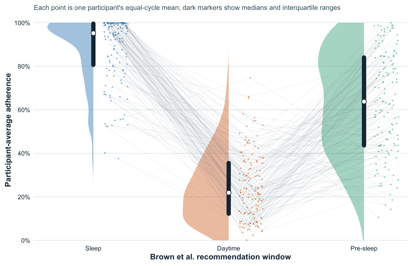
For participants represented in all three windows, each point is the participant's equal-cycle mean adherence. The lines connect the same participant's three summaries and are not time trajectories. The density shapes, median, and interquartile range describe this sample. Sleep reflects the bedside environment, rather than ocular exposure.
```{r}
#| label: association-profile-data
primary <- data.table::as.data.table(model_frames$primary_any_valid)
wake_consistency <- primary[, .(
  values = data.table::uniqueN(wake_fraction),
  minimum = min(wake_fraction),
  maximum = max(wake_fraction)
), by = .(participant_cluster, association_cycle_cluster)]
if (any(wake_consistency$values != 1L)) {
  stop("Wake adherence is not unique within participant-cycle.", call. = FALSE)
}

wake_cycle <- unique(primary[, .(
  participant_cluster,
  association_cycle_cluster,
  state = "Wake",
  adherence = wake_fraction
)])
target_cycle <- primary[, .(
  participant_cluster,
  association_cycle_cluster,
  state = as.character(target_state),
  adherence = target_fraction
)]

cycle_states <- data.table::rbindlist(list(wake_cycle, target_cycle))
profile_internal <- cycle_states[, .(
  mean_adherence = mean(adherence),
  valid_cycles = .N
), by = .(participant_cluster, state)]

state_levels <- c("Sleep", "Wake", "Pre-sleep")
state_display_labels <- c(
  "Sleep" = "Sleep",
  "Wake" = "Daytime",
  "Pre-sleep" = "Pre-sleep"
)
profile_internal[, state := factor(state, levels = state_levels)]
state_support_all <- profile_internal[, .(
  profiles = data.table::uniqueN(participant_cluster)
), by = .(state = as.character(state))]
profile_support <- profile_internal[, .(
  states_observed = data.table::uniqueN(state),
  sleep_observed = any(state == "Sleep"),
  wake_observed = any(state == "Wake"),
  pre_sleep_observed = any(state == "Pre-sleep")
), by = participant_cluster]
complete_clusters <- profile_support[states_observed == 3L, participant_cluster]
profile_internal <- profile_internal[participant_cluster %in% complete_clusters]
if (
  nrow(profile_internal) != length(complete_clusters) * 3L ||
    any(profile_internal[, .N, by = participant_cluster]$N != 3L)
) {
  stop("The complete profile display does not contain three-state profiles.", call. = FALSE)
}

# The sequential display key is assigned after a fixed arbitrary permutation.
# No cluster key or permutation map is written to disk.
set.seed(20260820L)
permuted_clusters <- sample(sort(complete_clusters), length(complete_clusters))
anonymous_key <- data.table::data.table(
  participant_cluster = permuted_clusters,
  profile_key = sprintf("profile_%03d", seq_along(permuted_clusters))
)
set.seed(20260821L)
anonymous_key[, point_offset := stats::runif(.N, min = 0.075, max = 0.255)]
profile_internal <- merge(
  profile_internal,
  anonymous_key,
  by = "participant_cluster",
  all.x = TRUE,
  sort = FALSE
)
profile_internal[, state_order := match(as.character(state), state_levels)]
profile_internal[, point_x := state_order + point_offset]
data.table::setorder(profile_internal, profile_key, state_order)

profile_source <- profile_internal[, .(
  profile_key,
  state = as.character(state),
  state_order,
  mean_adherence,
  valid_cycles,
  point_offset,
  point_x
)]
if (
  any(grepl("participant|cluster|site|rank|tertile", names(profile_source))) ||
    !all(grepl("^profile_[0-9]{3}$", profile_source$profile_key)) ||
    data.table::uniqueN(profile_source$profile_key) != length(complete_clusters) ||
    nrow(profile_source) != length(complete_clusters) * 3L
) {
  stop("The profile source failed its privacy or shape check.", call. = FALSE)
}
cs_write(profile_source, "participant_state_profiles_points.csv")

profile_summary <- profile_source[, .(
  profiles = .N,
  mean_adherence = mean(mean_adherence),
  standard_deviation = stats::sd(mean_adherence),
  median_adherence = stats::median(mean_adherence),
  lower_quartile = as.numeric(stats::quantile(mean_adherence, 0.25, type = 7)),
  upper_quartile = as.numeric(stats::quantile(mean_adherence, 0.75, type = 7)),
  minimum_adherence = min(mean_adherence),
  maximum_adherence = max(mean_adherence),
  median_valid_cycles = stats::median(valid_cycles),
  minimum_valid_cycles = min(valid_cycles),
  maximum_valid_cycles = max(valid_cycles)
), by = .(state, state_order)]
data.table::setorder(profile_summary, state_order)
cs_write(profile_summary, "participant_state_profiles_summary.csv")

sample_flow <- data.table::data.table(
  stage = c(
    "Any-valid association frame",
    "Participants represented in Sleep",
    "Participants represented in Wake",
    "Participants represented in Pre-sleep",
    "Complete three-state profile display",
    "Anonymous participant-state points"
  ),
  count = c(
    data.table::uniqueN(primary$participant_cluster),
    state_support_all[state == "Sleep", profiles],
    state_support_all[state == "Wake", profiles],
    state_support_all[state == "Pre-sleep", profiles],
    data.table::uniqueN(profile_source$profile_key),
    nrow(profile_source)
  ),
  unit = c("participants", "participants", "participants", "participants", "participants", "points")
)
cs_write(sample_flow, "participant_state_profiles_sample.csv")

knitr::kable(profile_summary)
```
```{r}
#| label: fig-association-profiles
#| fig-cap: "Participant-average recommendation adherence across Sleep, Daytime, and Pre-sleep. Dark markers show the median and interquartile range."
#| fig-alt: "Connected participant averages with density shapes for Sleep, Daytime, and Pre-sleep adherence. The connections identify the same anonymous participant across windows."
#| fig-width: 9.2
#| fig-height: 5.9
state_colors <- c(
  "Sleep" = "#0072B2",
  "Wake" = "#D55E00",
  "Pre-sleep" = "#009E73"
)
density_source <- data.table::rbindlist(lapply(
  seq_along(state_levels),
  function(index) {
    state_name <- state_levels[[index]]
    values <- profile_source[state == state_name, mean_adherence]
    estimate <- stats::density(
      values,
      from = 0,
      to = 1,
      n = 512,
      cut = 0,
      bw = "nrd0"
    )
    scaled <- estimate$y / max(estimate$y) * 0.34
    data.table::data.table(
      state = state_name,
      state_order = index,
      mean_adherence = c(0, estimate$x, 1),
      density_x = c(index, index - scaled, index)
    )
  }
))

plot_summary <- profile_summary[, .(
  state,
  state_order,
  median_percent = 100 * median_adherence,
  lower_quartile_percent = 100 * lower_quartile,
  upper_quartile_percent = 100 * upper_quartile
)]
plot_profiles <- data.table::copy(profile_source)
plot_profiles[, mean_adherence_percent := 100 * mean_adherence]

raincloud <- ggplot2::ggplot() +
  ggplot2::geom_polygon(
    data = density_source,
    ggplot2::aes(
      x = density_x,
      y = 100 * mean_adherence,
      group = state,
      fill = state
    ),
    alpha = 0.38,
    color = NA
  ) +
  ggplot2::geom_line(
    data = plot_profiles,
    ggplot2::aes(
      x = point_x,
      y = mean_adherence_percent,
      group = profile_key
    ),
    linewidth = 0.28,
    alpha = 0.11,
    color = "#526874"
  ) +
  ggplot2::geom_point(
    data = plot_profiles,
    ggplot2::aes(
      x = point_x,
      y = mean_adherence_percent,
      color = state
    ),
    size = 1.05,
    alpha = 0.55,
    stroke = 0
  ) +
  ggplot2::geom_linerange(
    data = plot_summary,
    ggplot2::aes(
      x = state_order,
      ymin = lower_quartile_percent,
      ymax = upper_quartile_percent
    ),
    linewidth = 3.2,
    color = "#173042",
    lineend = "round"
  ) +
  ggplot2::geom_point(
    data = plot_summary,
    ggplot2::aes(x = state_order, y = median_percent),
    shape = 21,
    size = 3.0,
    stroke = 0.7,
    fill = "white",
    color = "#173042"
  ) +
  ggplot2::scale_fill_manual(values = state_colors, guide = "none") +
  ggplot2::scale_color_manual(values = state_colors, guide = "none") +
  ggplot2::scale_x_continuous(
    breaks = seq_along(state_levels),
    labels = unname(state_display_labels[state_levels]),
    limits = c(0.56, 3.32),
    expand = ggplot2::expansion(mult = c(0, 0))
  ) +
  ggplot2::scale_y_continuous(
    breaks = seq(0, 100, 20),
    labels = function(value) paste0(value, "%"),
    limits = c(0, 100),
    expand = ggplot2::expansion(mult = c(0.01, 0.025))
  ) +
  ggplot2::labs(
    x = "Brown et al. recommendation window",
    y = "Participant-average adherence",
    subtitle = paste(
      "Each point is one participant's equal-cycle mean;",
      "dark markers show medians and interquartile ranges"
    )
  ) +
  ggplot2::theme_minimal(base_size = 12.5) +
  ggplot2::theme(
    plot.subtitle = ggplot2::element_text(
      color = "#445b68",
      size = 10.8,
      margin = ggplot2::margin(b = 10)
    ),
    axis.title = ggplot2::element_text(color = "#173042", face = "bold"),
    axis.text = ggplot2::element_text(color = "#173042"),
    panel.grid.major.x = ggplot2::element_blank(),
    panel.grid.minor = ggplot2::element_blank(),
    panel.grid.major.y = ggplot2::element_line(color = "#DCE5E9", linewidth = 0.35),
    plot.margin = ggplot2::margin(8, 14, 8, 8)
  )


cs_write(density_source, "participant_state_raincloud_density.csv")
cs_write(plot_profiles, "participant_state_raincloud_points.csv")
cs_write(plot_summary, "participant_state_raincloud_summary.csv")
dir.create("results/images/brown-association", recursive = TRUE, showWarnings = FALSE)
ggplot2::ggsave("results/images/brown-association/participant_state_raincloud.png", raincloud, device = ragg::agg_png, width = 9.2, height = 5.9, dpi = 320, background = "white")
ggplot2::ggsave("results/images/brown-association/participant_state_raincloud.svg", raincloud, device = svglite::svglite, width = 9.2, height = 5.9, bg = "white")
raincloud
```
## Interpretation
The within-participant differences are `r sprintf("%.2f", effect_source[association_level == "within" & target_state == "Sleep", response_effect_percentage_points])` percentage points for Sleep and `r sprintf("%.2f", effect_source[association_level == "within" & target_state == "Pre-sleep", response_effect_percentage_points])` for Pre-sleep per ten percentage points higher-than-usual daytime adherence. Both intervals include zero. The within-participant inference remains qualified by unresolved temporal dependence.
Between participants, the corresponding differences are `r sprintf("%.2f", effect_source[association_level == "between" & target_state == "Sleep", response_effect_percentage_points])` percentage points for Sleep and `r sprintf("%.2f", effect_source[association_level == "between" & target_state == "Pre-sleep", response_effect_percentage_points])` for Pre-sleep. The negative associations indicate lower target-window adherence among participants with higher observed average daytime adherence; they do not identify the direction of causation.
The model separates within- and between-participant associations over the observed monitoring period. Interval exclusion and FDR-adjusted testing answer different questions, and model adequacy constrains both. Residual temporal dependence and failures in the temporal sensitivity fits qualify within-participant interpretation. Between-participant associations remain observational and may reflect measured or unmeasured differences between participants. The underlying numeric estimates, covariance matrices, model checks, sensitivity comparisons, and exact figure data are regenerated under `results/`.