---
title: "H02: Daily patterns of personal light exposure"
engine: knitr
execute:
echo: true
format:
html:
toc: true
code-fold: false
---
## Question and analysis sequence
This analysis models 30-minute near-eye light exposure across the day. It
separates the common daily curve from variation between sites, participants,
and participant-days. Chest measurements, placement-matched observations,
alternative preprocessing, and alternative smooth specifications assess the
sensitivity of the findings.
The inputs are generated by the preparation pages. This notebook constructs
the fitted samples, estimates the models, evaluates temporal assumptions,
and exports numerical estimates and the data underlying the figures.
## Data and model guide {#methods}
The [analysis datasets](../preparation/06-analysis-datasets.qmd) provide
30-minute arithmetic-mean melanopic EDI. A primary bin requires at least 15 valid
one-minute observations. Exact zeros remain observations; unsupported bins remain
missing. The response is `log10(melEDI + 0.1)`. All-available and matched-bin samples
are constructed separately for the two sensor positions and preprocessing datasets.
The model separates a shared local-clock curve, sum-to-zero site deviations,
participant-specific curves and participant-day intercepts. The shared curve is
cyclic at midnight. An additional sensitivity also makes the site and participant
deviations cyclic. Local wall time describes daily shape, while true elapsed time
orders residual sequences. AR(1) sequences restart at participant-day boundaries,
missing half-hours and ambiguous elapsed-time links. Each scenario estimates its
own AR parameter from a preliminary fit; the final model uses the verified boundaries.
Fitted-curve dispersion and Shapley allocation answer different questions. Dispersion
compares the spread of fitted site, participant and day components. Shapley allocation
averages contributions across component subsets to allocate in-sample R². Ratios of
participant to site contributions are reported for each measure. Hierarchical
bootstrap intervals condition on the fitted model; they are not joint model-refit
intervals. Clock-specific curve intervals are pointwise, not simultaneous bands.
The subsequent sections show exact formulas, sample support, residual checks,
matched-placement comparisons and alternative preprocessing.
The executable sections below write fitted objects to `results/models/H02/`,
reader tables to `results/tables/H02/`, and the supporting numerical and figure
outputs under `results/`. Start with the calculations below or jump to
[findings and interpretation](#findings).
## Libraries and shared settings
```{r}
#| label: h02-analysis-setup
library(dplyr)
library(tidyr)
library(tibble)
library(readr)
library(ggplot2)
library(mgcv)
library(gt)
source("scripts/project.R")
analysis_setup()
root <- getOption("nh.root")
source("scripts/pipeline/paths_io.R")
source("scripts/pipeline/assertions.R")
source("scripts/pipeline/multiplicity.R")
source("scripts/hypotheses/H02/h02_contract.R")
source("scripts/hypotheses/H02/h02_data.R")
source("scripts/hypotheses/H02/h02_modeling.R")
source("scripts/hypotheses/H02/h02_dominance.R")
source("scripts/hypotheses/H02/h02_result_helpers.R")
paths <- pipeline_paths(root)
producer <- "analyses/H02-daily-patterns.qmd"
for (directory in file.path(c(paths$models, paths$diagnostics, paths$tables,
                             paths$figures, paths$source_data), "H02")) {
  dir.create(directory, recursive = TRUE, showWarnings = FALSE)
}
h02_validate_inputs(root)
```
## Construct the analysis samples
Join local-clock bins to their true elapsed-time sequence. Gaps and discontinuities define separate autocorrelation sequences. The alternative preprocessing and placement-matched samples use the same model-frame rules.
```{r}
#| label: h02-analysis-samples
links <- h02_temporal_links(root)
h02_assert_temporal_links(links)

input <- h02_input_contract(root)
input_path <- function(id) input$path[match(id, input$input_id)]

main_gr_grid <- h02_main_grid(
  input_path("main_glasses"),
  "main",
  links
)
main_ch_grid <- h02_main_grid(
  input_path("main_chest"),
  "main",
  links
)
alternative_all <- h02_alternative_grid(
  input_path("alternative_preprocessing"),
  links
)
mp_gr_grid <- dplyr::filter(alternative_all, .data$position == "glasses")
mp_ch_grid <- dplyr::filter(alternative_all, .data$position == "chest")

frames <- list(
  main = list(
    glasses = h02_model_frame(main_gr_grid),
    chest = h02_model_frame(main_ch_grid)
  ),
  alternative_preprocessing = list(
    glasses = h02_model_frame(mp_gr_grid),
    chest = h02_model_frame(mp_ch_grid)
  )
)
for (scenario in names(frames)) {
  paired <- h02_paired_frames(
    frames[[scenario]]$glasses,
    frames[[scenario]]$chest
  )
  frames[[scenario]]$paired_common_sample <- paired
}

registry <- h02_run_registry()
frame_for_run <- function(scenario, placement, sample) {
  if (sample == "all_available") {
    frames[[scenario]][[placement]]
  } else {
    frames[[scenario]]$paired_common_sample[[placement]]
  }
}

model_data_dir <- file.path(paths$model_data, "H02")
dir.create(model_data_dir, recursive = TRUE, showWarnings = FALSE)
for (i in seq_len(nrow(registry))) {
  run <- registry[i, ]
  frame <- frame_for_run(run$data_scenario_id, run$placement, run$sample_scenario)
  write_h02_rds(frame, file.path(model_data_dir, paste0(run$run_id, ".rds")))
}
sample_counts <- purrr::pmap_dfr(
  registry[c("data_scenario_id", "placement", "sample_scenario", "run_id")],
  function(data_scenario_id, placement, sample_scenario, run_id) {
    h02_sample_counts(
      frame_for_run(data_scenario_id, placement, sample_scenario),
      run_id
    )
  }
)
support_audit <- dplyr::bind_rows(
  h02_support_audit(main_gr_grid, "main", "glasses"),
  h02_support_audit(main_ch_grid, "main", "chest"),
  h02_support_audit(
    mp_gr_grid,
    "alternative_preprocessing",
    "glasses"
  ),
  h02_support_audit(
    mp_ch_grid,
    "alternative_preprocessing",
    "chest"
  )
)

comparison <- dplyr::full_join(
  frames$main$glasses |>
    dplyr::select(
      dplyr::all_of(h02_key),
      main_metric_value_lx = "metric_value_lx"
    ),
  frames$alternative_preprocessing$glasses |>
    dplyr::select(
      dplyr::all_of(h02_key),
      alternative_metric_value_lx = "metric_value_lx"
    ),
  by = h02_key,
  relationship = "one-to-one"
) |>
  dplyr::mutate(position = "glasses")
comparison_chest <- dplyr::full_join(
  frames$main$chest |>
    dplyr::select(
      dplyr::all_of(h02_key),
      main_metric_value_lx = "metric_value_lx"
    ),
  frames$alternative_preprocessing$chest |>
    dplyr::select(
      dplyr::all_of(h02_key),
      alternative_metric_value_lx = "metric_value_lx"
    ),
  by = h02_key,
  relationship = "one-to-one"
) |>
  dplyr::mutate(position = "chest")
scenario_input_comparison <- dplyr::bind_rows(comparison, comparison_chest) |>
  dplyr::group_by(.data$position) |>
  dplyr::summarise(
    main_finite = sum(is.finite(.data$main_metric_value_lx)),
    alternative_finite = sum(is.finite(.data$alternative_metric_value_lx)),
    common_finite = sum(
      is.finite(.data$main_metric_value_lx) &
        is.finite(.data$alternative_metric_value_lx)
    ),
    exactly_equal_common = sum(
      is.finite(.data$main_metric_value_lx) &
        is.finite(.data$alternative_metric_value_lx) &
        .data$main_metric_value_lx == .data$alternative_metric_value_lx
    ),
    mean_main_minus_alternative_lx = mean(
      .data$main_metric_value_lx - .data$alternative_metric_value_lx,
      na.rm = TRUE
    ),
    max_absolute_difference_lx = max(
      abs(.data$main_metric_value_lx - .data$alternative_metric_value_lx),
      na.rm = TRUE
    ),
    .groups = "drop"
  )

tables <- list(sample_counts = sample_counts, support_audit = support_audit,
               scenario_input_comparison = scenario_input_comparison,
               temporal_model_specification = h02_specification_table())
for (name in names(tables)) {
  write_h02_csv(tables[[name]], file.path(model_data_dir, paste0(name, ".csv")))
}
sample_counts |> gt()
```
## Fit daily patterns and quantify variation
Select the temporal structure using the primary near-eye sample, estimate residual autocorrelation, and fit the selected structure to each sensitivity sample. Bootstrap intervals resample sites, participants, and participant-days from fitted contributions; full reproduction uses 2,000 replicates.
```{r}
#| label: h02-fit-daily-patterns
registry <- h02_run_registry() |>
  dplyr::mutate(
    run_order = dplyr::case_when(
      .data$analytical_role == "primary" ~ 1L,
      .data$analytical_role == "alternative_preprocessing_sensitivity" ~ 2L,
      .data$data_scenario_id == "main" &
        .data$placement == "chest" &
        .data$sample_scenario == "all_available" ~
        3L,
      .data$data_scenario_id == "alternative_preprocessing" &
        .data$placement == "chest" &
        .data$sample_scenario == "all_available" ~
        4L,
      .data$data_scenario_id == "main" ~ 5L,
      TRUE ~ 6L
    )
  ) |>
  dplyr::arrange(.data$run_order, .data$run_id)

model_tables <- list()
comparison_tables <- list()
residual_acf_tables <- list()
residual_summary_tables <- list()
boundary_tables <- list()
k_check_tables <- list()
influence_score_tables <- list()
contribution_influence_tables <- list()
site_prediction_tables <- list()
variation_tables <- list()
selected_model_id <- NULL
primary_rho <- NA_real_

for (i in seq_len(nrow(registry))) {
  run <- registry[i, ]
  run_id <- run$run_id
  message(
    "Fitting H02 run ",
    i,
    "/",
    nrow(registry),
    ": ",
    run_id
  )
  frame_path <- file.path(
    paths$model_data,
    "H02",
    paste0(run_id, ".rds")
  )
  if (!file.exists(frame_path)) {
    h02_abort(
      "Missing H02 model frame %s; execute the preceding analysis-sample section first",
      frame_path
    )
  }
  frame <- readRDS(frame_path)

  if (run$analytical_role == "primary") {
    fitted <- h02_fit_primary_structure(frame, run_id)
    selected_model_id <- fitted$selected_model_id
    primary_rho <- fitted$rho
    model_tables[[run_id]] <- dplyr::bind_rows(
      fitted$model_table,
      h02_model_row(
        fitted$final,
        paste0(selected_model_id, "_final_fREML"),
        run_id,
        fitted$rho
      )
    )
    comparison_tables[[run_id]] <- fitted$comparisons
  } else {
    if (is.null(selected_model_id)) {
      h02_abort("Primary H02 model must be selected before sensitivities")
    }
    fitted <- h02_fit_selected_run(
      frame,
      run_id,
      selected_model_id
    )
    model_tables[[run_id]] <- fitted$model_table
  }

  residual_acf_tables[[run_id]] <- dplyr::bind_rows(
    h02_residual_acf(
      fitted$preliminary,
      fitted$data,
      "preliminary_no_AR1",
      run_id
    ),
    h02_residual_acf(
      fitted$final,
      fitted$data,
      "final_AR1_standardized",
      run_id
    )
  )
  residual_summary_tables[[run_id]] <- h02_residual_summary(
    fitted$final,
    fitted$data,
    run_id
  )
  boundary_tables[[run_id]] <- h02_boundary_audit(
    fitted$data,
    run_id
  )
  k_check_tables[[run_id]] <- h02_k_check(fitted$final, run_id)
  influence_score_tables[[run_id]] <- h02_influence_scores(
    fitted$final,
    fitted$data,
    run_id
  )

  site_predictions <- h02_site_predictions(
    fitted$final,
    fitted$data,
    run_id
  )
  variation <- h02_variation_summary(
    fitted$final,
    fitted$data,
    site_predictions,
    run_id
  )
  site_prediction_tables[[run_id]] <- site_predictions
  variation_tables[[run_id]] <- variation$summary

  if (run$analytical_role == "primary") {
    contribution_influence_tables[[run_id]] <-
      h02_contribution_influence(
        variation$contributions,
        variation$summary,
        run_id
      )
  }

  model_diagnostics <- list(
    run_id = run_id,
    selected_model_id = selected_model_id,
    rho = fitted$rho,
    model_table = model_tables[[run_id]],
    comparisons = comparison_tables[[run_id]],
    residual_acf = residual_acf_tables[[run_id]],
    residual_summary = residual_summary_tables[[run_id]],
    boundary_audit = boundary_tables[[run_id]],
    k_check = k_check_tables[[run_id]],
    influence_scores = influence_score_tables[[run_id]],
    contribution_influence = contribution_influence_tables[[run_id]],
    site_predictions = site_prediction_tables[[run_id]],
    variation_summary = variation_tables[[run_id]]
  )
  write_h02_rds(
    model_diagnostics,
    file.path(
      paths$diagnostics,
      "H02",
      paste0(run_id, "__model_diagnostics.rds")
    ),
    paste0(run_id, "__model_diagnostics")
  )
  model_path <- file.path(
    paths$models,
    "H02",
    paste0(run_id, "__selected_model.rds")
  )
  write_h02_rds(
    fitted$final,
    model_path,
    paste0(run_id, "__model"),
    metadata = list(
      run_id = run_id,
      selected_model_id = selected_model_id,
      rho = fitted$rho,
      participants = dplyr::n_distinct(fitted$data$participant),
      participant_days = dplyr::n_distinct(fitted$data$participant_day),
      observations = nrow(fitted$data),
      sites = dplyr::n_distinct(fitted$data$site)
    )
  )
  write_h02_rds(
    variation$contributions,
    file.path(
      paths$source_data,
      "H02",
      paste0(run_id, "__fitted_contributions.rds")
    ),
    paste0(run_id, "__contributions")
  )
  write_h02_rds(
    variation$bootstrap,
    file.path(
      paths$diagnostics,
      "H02",
      paste0(run_id, "__variation_bootstrap.rds")
    ),
    paste0(run_id, "__variation_bootstrap")
  )
  rm(variation, site_predictions, frame)
  if (!is.null(fitted$candidates)) {
    fitted$candidates <- NULL
  }
  rm(fitted)
  invisible(gc())
}
bind_rows(variation_tables) |> filter(run_id == "main__glasses__all_available") |> gt()
```
## Compare sites and preprocessing choices
Apply the registered one-test omnibus family and compare the variation estimates between the two preprocessing variants. Simultaneous intervals describe where site curves differ from the equal-site mean.
```{r}
#| label: h02-inference-and-preprocessing
model_table <- dplyr::bind_rows(model_tables)
comparison_table <- dplyr::bind_rows(comparison_tables) |>
  dplyr::mutate(
    family_id = dplyr::if_else(
      .data$comparison_id == "site_pattern_vs_no_site",
      "H02-F1-site-pattern",
      NA_character_
    ),
    family_n = dplyr::if_else(
      .data$comparison_id == "site_pattern_vs_no_site",
      1L,
      NA_integer_
    ),
    adjustment_method = dplyr::if_else(
      .data$comparison_id == "site_pattern_vs_no_site",
      "BH",
      NA_character_
    ),
    inferential_role = dplyr::if_else(
      .data$comparison_id == "site_pattern_vs_no_site",
      "single registered omnibus site-pattern family",
      paste(
        "restricted-likelihood structure diagnostic;",
        "no multiplicity claim"
      )
    )
  )
comparison_table$p_adjusted <- NA_real_
family_rows <- which(
  comparison_table$comparison_id == "site_pattern_vs_no_site"
)
comparison_table$p_adjusted[family_rows] <- adjust_p_family(
  comparison_table$p_raw[family_rows],
  method = "BH",
  n = 1L
)
residual_acf <- dplyr::bind_rows(residual_acf_tables)
residual_summary <- dplyr::bind_rows(residual_summary_tables)
boundary_audit <- dplyr::bind_rows(boundary_tables)
k_check <- dplyr::bind_rows(k_check_tables)
influence_scores <- dplyr::bind_rows(influence_score_tables)
contribution_influence <- dplyr::bind_rows(
  contribution_influence_tables
)
site_predictions <- dplyr::bind_rows(site_prediction_tables)
variation_summary <- dplyr::bind_rows(variation_tables)
site_windows <- dplyr::bind_rows(lapply(
  unique(site_predictions$run_id),
  function(run_id) h02_site_windows(site_predictions, run_id)
))

primary_id <- "main__glasses__all_available"
alternative_id <-
  "alternative_preprocessing__glasses__all_available"
primary_variation <- dplyr::filter(
  variation_summary,
  .data$run_id == primary_id
)
alternative_variation <- dplyr::filter(
  variation_summary,
  .data$run_id == alternative_id
)
stability <- dplyr::inner_join(
  primary_variation |>
    dplyr::transmute(
      summary_id = .data$summary_id,
      main_estimate = .data$estimate,
      main_lower_95 = .data$lower_95,
      main_upper_95 = .data$upper_95
    ),
  alternative_variation |>
    dplyr::transmute(
      summary_id = .data$summary_id,
      alternative_estimate = .data$estimate,
      alternative_lower_95 = .data$lower_95,
      alternative_upper_95 = .data$upper_95
    ),
  by = "summary_id",
  relationship = "one-to-one"
) |>
  dplyr::mutate(
    relative_change = (.data$alternative_estimate - .data$main_estimate) /
      .data$main_estimate,
    confidence_intervals_overlap = pmax(
      .data$main_lower_95,
      .data$alternative_lower_95
    ) <=
      pmin(.data$main_upper_95, .data$alternative_upper_95),
    ratio_summary = grepl("ratio$", .data$summary_id),
    main_relation_to_one = dplyr::case_when(
      !.data$ratio_summary ~ "not_applicable",
      .data$main_lower_95 > 1 ~ "above_one",
      .data$main_upper_95 < 1 ~ "below_one",
      TRUE ~ "includes_one"
    ),
    alternative_relation_to_one = dplyr::case_when(
      !.data$ratio_summary ~ "not_applicable",
      .data$alternative_lower_95 > 1 ~ "above_one",
      .data$alternative_upper_95 < 1 ~ "below_one",
      TRUE ~ "includes_one"
    ),
    stability_classification = dplyr::case_when(
      .data$ratio_summary &
        sign(.data$main_estimate - 1) != sign(.data$alternative_estimate - 1) ~
        "unstable",
      .data$ratio_summary &
        .data$main_relation_to_one != .data$alternative_relation_to_one ~
        "inference-sensitive",
      abs(.data$relative_change) <= 0.20 &
        .data$confidence_intervals_overlap ~
        "stable",
      abs(.data$relative_change) <= 0.50 &
        .data$confidence_intervals_overlap ~
        "directionally stable",
      TRUE ~ "magnitude-sensitive"
    ),
    scenario_change = paste(
      "Only the prepared dataset changed; formula, transformation, basis",
      "dimensions, structure, selection result, rho-estimation algorithm,",
      "AR-boundary algorithm, summaries, and CI algorithm were identical."
    )
  )

primary_window_summary <- site_windows |>
  dplyr::filter(.data$run_id == primary_id) |>
  dplyr::mutate(
    window_text = dplyr::if_else(
      .data$direction == "no_simultaneous_difference",
      "No 30-minute bin had a simultaneous 95% interval excluding 1",
      sprintf(
        "%s %s-%s; point-ratio range %.2f-%.2f",
        .data$direction,
        .data$start_local_clock,
        .data$end_local_clock,
        .data$minimum_point_ratio,
        .data$maximum_point_ratio
      )
    )
  ) |>
  dplyr::group_by(.data$site) |>
  dplyr::summarise(
    new_H02_simultaneous_result = paste(
      .data$window_text,
      collapse = "; "
    ),
    .groups = "drop"
  )
selected_specification <- h02_selected_model_specification(
  readRDS(file.path(
    paths$models,
    "H02",
    paste0(primary_id, "__selected_model.rds")
  )),
  selected_model_id,
  primary_rho,
  primary_id
)
comparison_table |> gt()
stability |> select(summary_id, main_estimate, alternative_estimate, stability_classification) |> gt()
```
## Export numerical results and inspect the primary curves
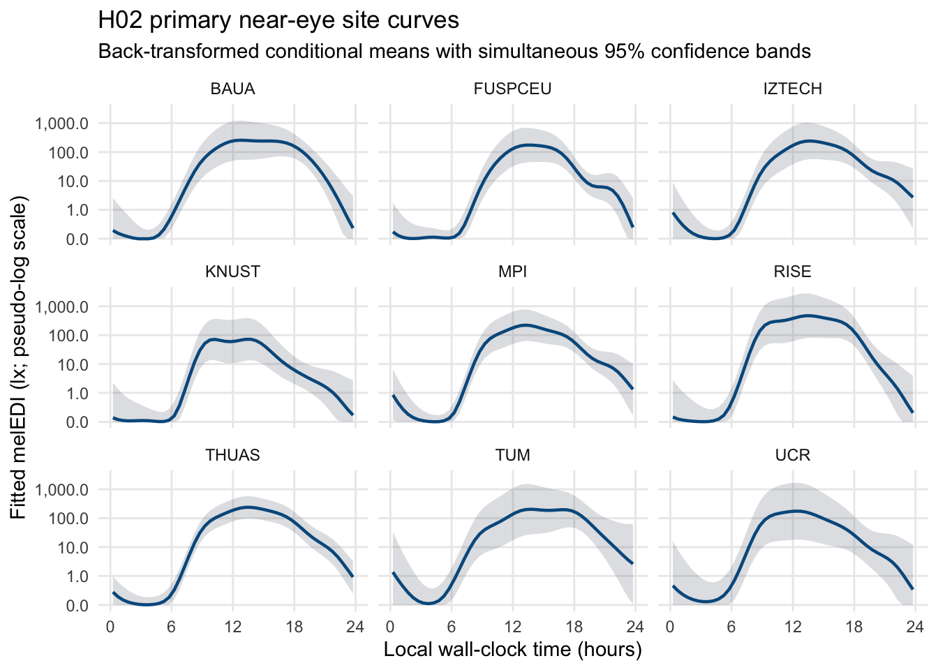
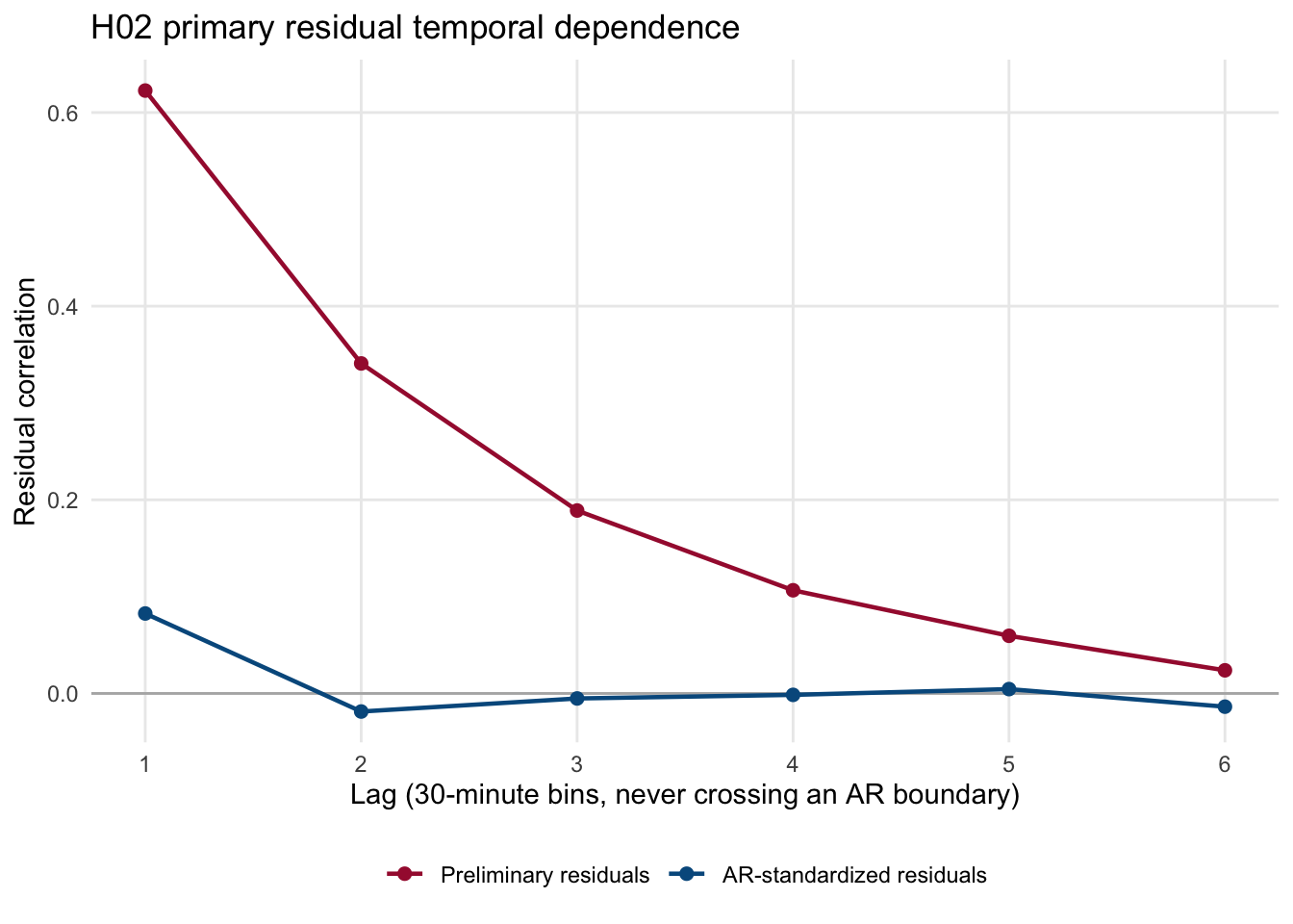
Save estimates, diagnostics, and exact curve data. The figures display the fitted site curves and the residual correlation remaining after accounting for elapsed-time sequences.
```{r}
#| label: h02-export-and-curves
tables <- list(
  model_fit_summary = model_table,
  model_structure_comparisons = comparison_table,
  residual_acf = residual_acf,
  residual_summary = residual_summary,
  ar_boundary_audit = boundary_audit,
  basis_dimension_checks = k_check,
  influence_scores = influence_scores,
  conditional_deletion_influence = contribution_influence,
  variation_summary = variation_summary,
  alternative_preprocessing_stability = stability,
  simultaneous_site_windows = site_windows,
  selected_temporal_model_specification = selected_specification
)
table_locations <- c(
  model_fit_summary = file.path(
    paths$tables,
    "H02",
    "model_fit_summary.csv"
  ),
  model_structure_comparisons = file.path(
    paths$tables,
    "H02",
    "model_structure_comparisons.csv"
  ),
  residual_acf = file.path(
    paths$diagnostics,
    "H02",
    "residual_acf.csv"
  ),
  residual_summary = file.path(
    paths$diagnostics,
    "H02",
    "residual_summary.csv"
  ),
  ar_boundary_audit = file.path(
    paths$diagnostics,
    "H02",
    "ar_boundary_audit.csv"
  ),
  basis_dimension_checks = file.path(
    paths$diagnostics,
    "H02",
    "basis_dimension_checks.csv"
  ),
  influence_scores = file.path(
    paths$diagnostics,
    "H02",
    "influence_scores.csv"
  ),
  conditional_deletion_influence = file.path(
    paths$diagnostics,
    "H02",
    "conditional_deletion_influence.csv"
  ),
  variation_summary = file.path(
    paths$tables,
    "H02",
    "variation_summary.csv"
  ),
  alternative_preprocessing_stability = file.path(
    paths$tables,
    "H02",
    "alternative_preprocessing_stability.csv"
  ),
  simultaneous_site_windows = file.path(
    paths$tables,
    "H02",
    "simultaneous_site_windows.csv"
  ),
  selected_temporal_model_specification = file.path(
    paths$models,
    "H02",
    "selected_temporal_model_specification.csv"
  )
)
for (name in names(tables)) {
  write_h02_csv(
    tables[[name]],
    table_locations[[name]],
    paste0("table__", name)
  )
}

write_h02_csv(
  site_predictions,
  file.path(paths$source_data, "H02", "site_curve_predictions.csv"),
  "source__site_curve_predictions"
)

primary_curves <- dplyr::filter(
  site_predictions,
  .data$run_id == primary_id
)
curve_plot <- ggplot(
  primary_curves,
  aes(x = .data$time_hour, y = .data$estimate_melEDI_lx)
) +
  geom_ribbon(
    aes(
      ymin = .data$lower_melEDI_lx,
      ymax = .data$upper_melEDI_lx
    ),
    fill = "#6B7280",
    alpha = 0.22
  ) +
  geom_line(colour = "#005A8D", linewidth = 0.8) +
  facet_wrap(vars(.data$site), ncol = 3) +
  scale_x_continuous(
    breaks = seq(0, 24, by = 6),
    limits = c(0, 24)
  ) +
  scale_y_continuous(
    trans = scales::pseudo_log_trans(base = 10, sigma = 0.1),
    breaks = c(0, 1, 10, 100, 1000),
    labels = scales::label_number(big.mark = ",")
  ) +
  labs(
    x = "Local wall-clock time (hours)",
    y = "Fitted melEDI (lx; pseudo-log scale)",
    title = "H02 primary near-eye site curves",
    subtitle = paste(
      "Back-transformed conditional means with simultaneous 95%",
      "confidence bands"
    )
  ) +
  theme_minimal(base_size = 11) +
  theme(panel.grid.minor = element_blank())
write_h02_plot(
  curve_plot,
  file.path(paths$figures, "H02", "primary_site_curves.png"),
  "figure__primary_site_curves",
  width = 10,
  height = 8
)

acf_plot_data <- residual_acf |>
  dplyr::filter(.data$run_id == primary_id)
acf_plot <- ggplot(
  acf_plot_data,
  aes(
    x = .data$lag_30_minute_bins,
    y = .data$correlation,
    colour = .data$stage
  )
) +
  geom_hline(yintercept = 0, colour = "grey70") +
  geom_line(linewidth = 0.8) +
  geom_point(size = 2) +
  scale_x_continuous(breaks = seq_len(6L)) +
  scale_colour_manual(
    values = c(
      preliminary_no_AR1 = "#A61C3C",
      final_AR1_standardized = "#005A8D"
    ),
    breaks = c(
      "preliminary_no_AR1",
      "final_AR1_standardized"
    ),
    labels = c(
      "Preliminary residuals",
      "AR-standardized residuals"
    )
  ) +
  labs(
    x = "Lag (30-minute bins, never crossing an AR boundary)",
    y = "Residual correlation",
    colour = NULL,
    title = "H02 primary residual temporal dependence"
  ) +
  theme_minimal(base_size = 11) +
  theme(legend.position = "bottom", panel.grid.minor = element_blank())
write_h02_plot(
  acf_plot,
  file.path(paths$figures, "H02", "primary_residual_acf.png"),
  "figure__primary_residual_acf",
  width = 7,
  height = 4.5
)
curve_plot
acf_plot
```
## Sensitivity to the site-smooth specification
Replace the primary sum-to-zero site smooths with ordered cyclic difference smooths. The response, sample, autocorrelation algorithm, and summaries are held fixed.
```{r}
#| label: h02-cyclic-formula-sensitivity
formula_id <- "cyclic_ordered_sensitivity"
scenarios <- tibble::tribble(
  ~data_scenario_id,
  ~base_run_id,
  "main",
  "main__glasses__all_available",
  "alternative_preprocessing",
  "alternative_preprocessing__glasses__all_available"
) |>
  dplyr::mutate(
    sensitivity_run_id = paste0(
      .data$base_run_id,
      "__",
      formula_id
    )
  )

model_tables <- list()
variation_tables <- list()
residual_acf_tables <- list()
residual_summary_tables <- list()
k_check_tables <- list()
site_prediction_tables <- list()

for (i in seq_len(nrow(scenarios))) {
  scenario <- scenarios[i, ]
  message(
    "Fitting H02 formula sensitivity ",
    i,
    "/",
    nrow(scenarios),
    ": ",
    scenario$sensitivity_run_id
  )
  frame <- readRDS(file.path(
    paths$model_data,
    "H02",
    paste0(scenario$base_run_id, ".rds")
  ))
  fitted <- h02_fit_selected_run(
    frame,
    scenario$sensitivity_run_id,
    formula_id
  )
  predictions <- h02_site_predictions(
    fitted$final,
    fitted$data,
    scenario$sensitivity_run_id
  )
  variation <- h02_variation_summary(
    fitted$final,
    fitted$data,
    predictions,
    scenario$sensitivity_run_id
  )

  model_tables[[scenario$sensitivity_run_id]] <- fitted$model_table |>
    dplyr::mutate(
      data_scenario_id = scenario$data_scenario_id,
      formula_role = "model-form sensitivity",
      .before = 1L
    )
  variation_tables[[scenario$sensitivity_run_id]] <- variation$summary |>
    dplyr::mutate(
      data_scenario_id = scenario$data_scenario_id,
      formula_role = "model-form sensitivity",
      .before = 1L
    )
  residual_acf_tables[[scenario$sensitivity_run_id]] <- dplyr::bind_rows(
    h02_residual_acf(
      fitted$preliminary,
      fitted$data,
      "preliminary_no_AR1",
      scenario$sensitivity_run_id
    ),
    h02_residual_acf(
      fitted$final,
      fitted$data,
      "final_AR1_standardized",
      scenario$sensitivity_run_id
    )
  ) |>
    dplyr::mutate(
      data_scenario_id = scenario$data_scenario_id,
      .before = 1L
    )
  residual_summary_tables[[scenario$sensitivity_run_id]] <-
    h02_residual_summary(
      fitted$final,
      fitted$data,
      scenario$sensitivity_run_id
    ) |>
    dplyr::mutate(
      data_scenario_id = scenario$data_scenario_id,
      .before = 1L
    )
  k_check_tables[[scenario$sensitivity_run_id]] <- h02_k_check(
    fitted$final,
    scenario$sensitivity_run_id
  ) |>
    dplyr::mutate(
      data_scenario_id = scenario$data_scenario_id,
      .before = 1L
    )
  site_prediction_tables[[scenario$sensitivity_run_id]] <- predictions |>
    dplyr::mutate(
      data_scenario_id = scenario$data_scenario_id,
      .before = 1L
    )

  write_h02_rds(
    fitted$final,
    file.path(
      paths$models,
      "H02",
      paste0(scenario$sensitivity_run_id, "__selected_model.rds")
    ),
    paste0(scenario$sensitivity_run_id, "__model"),
    metadata = list(
      base_run_id = scenario$base_run_id,
      formula_id = formula_id,
      rho = fitted$rho,
      participants = dplyr::n_distinct(fitted$data$participant),
      participant_days = dplyr::n_distinct(fitted$data$participant_day),
      observations = nrow(fitted$data),
      sites = dplyr::n_distinct(fitted$data$site)
    )
  )
  write_h02_rds(
    variation$contributions,
    file.path(
      paths$source_data,
      "H02",
      paste0(scenario$sensitivity_run_id, "__fitted_contributions.rds")
    ),
    paste0(scenario$sensitivity_run_id, "__contributions")
  )
  write_h02_rds(
    variation$bootstrap,
    file.path(
      paths$diagnostics,
      "H02",
      paste0(scenario$sensitivity_run_id, "__variation_bootstrap.rds")
    ),
    paste0(scenario$sensitivity_run_id, "__variation_bootstrap")
  )
  rm(frame, fitted, predictions, variation)
  invisible(gc())
}
model_summary <- dplyr::bind_rows(model_tables)
variation_summary <- dplyr::bind_rows(variation_tables)
residual_acf <- dplyr::bind_rows(residual_acf_tables)
residual_summary <- dplyr::bind_rows(residual_summary_tables)
k_check <- dplyr::bind_rows(k_check_tables)
site_predictions <- dplyr::bind_rows(site_prediction_tables)

primary_variation <- readr::read_csv(
  file.path(paths$tables, "H02", "variation_summary.csv"),
  show_col_types = FALSE
) |>
  dplyr::filter(.data$run_id %in% scenarios$base_run_id) |>
  dplyr::inner_join(
    scenarios |>
      dplyr::select("data_scenario_id", "base_run_id"),
    by = c("run_id" = "base_run_id"),
    relationship = "many-to-one"
  )

comparison <- dplyr::inner_join(
  primary_variation |>
    dplyr::transmute(
      data_scenario_id = .data$data_scenario_id,
      summary_id = .data$summary_id,
      primary_sz_estimate = .data$estimate,
      primary_sz_lower_95 = .data$lower_95,
      primary_sz_upper_95 = .data$upper_95
    ),
  variation_summary |>
    dplyr::transmute(
      data_scenario_id = .data$data_scenario_id,
      summary_id = .data$summary_id,
      cyclic_sensitivity_estimate = .data$estimate,
      cyclic_sensitivity_lower_95 = .data$lower_95,
      cyclic_sensitivity_upper_95 = .data$upper_95
    ),
  by = c("data_scenario_id", "summary_id"),
  relationship = "one-to-one"
) |>
  dplyr::mutate(
    relative_change = (.data$cyclic_sensitivity_estimate -
      .data$primary_sz_estimate) /
      .data$primary_sz_estimate,
    confidence_intervals_overlap = pmax(
      .data$primary_sz_lower_95,
      .data$cyclic_sensitivity_lower_95
    ) <=
      pmin(
        .data$primary_sz_upper_95,
        .data$cyclic_sensitivity_upper_95
      ),
    ratio_summary = grepl("ratio$", .data$summary_id),
    primary_relation_to_one = dplyr::case_when(
      !.data$ratio_summary ~ "not_applicable",
      .data$primary_sz_lower_95 > 1 ~ "above_one",
      .data$primary_sz_upper_95 < 1 ~ "below_one",
      TRUE ~ "includes_one"
    ),
    sensitivity_relation_to_one = dplyr::case_when(
      !.data$ratio_summary ~ "not_applicable",
      .data$cyclic_sensitivity_lower_95 > 1 ~ "above_one",
      .data$cyclic_sensitivity_upper_95 < 1 ~ "below_one",
      TRUE ~ "includes_one"
    ),
    stability_classification = dplyr::case_when(
      .data$ratio_summary &
        sign(.data$primary_sz_estimate - 1) !=
          sign(.data$cyclic_sensitivity_estimate - 1) ~
        "unstable",
      .data$ratio_summary &
        .data$primary_relation_to_one != .data$sensitivity_relation_to_one ~
        "inference-sensitive",
      abs(.data$relative_change) <= 0.20 &
        .data$confidence_intervals_overlap ~
        "stable",
      abs(.data$relative_change) <= 0.50 &
        .data$confidence_intervals_overlap ~
        "directionally stable",
      TRUE ~ "magnitude-sensitive"
    ),
    scenario_change = paste(
      "Only the model formula and associated basis dimensions changed:",
      "primary overall cc(k=12) + site sz(k=12) + participant fs(k=10)",
      "versus cyclic sensitivity with parametric site + overall cc(k=12) +",
      "ordered-factor site cc(k=12,id=1) + participant fs(cc,k=8);",
      "data, transform, rho algorithm, AR boundaries, summaries, and",
      "conditional interval algorithm were identical."
    )
  )

tables <- list(
  formula_sensitivity_model_fit_summary = model_summary,
  formula_sensitivity_variation_summary = variation_summary,
  formula_sensitivity_comparison = comparison,
  formula_sensitivity_residual_acf = residual_acf,
  formula_sensitivity_residual_summary = residual_summary,
  formula_sensitivity_basis_dimension_checks = k_check
)
table_locations <- c(
  formula_sensitivity_model_fit_summary = file.path(
    paths$tables,
    "H02",
    "formula_sensitivity_model_fit_summary.csv"
  ),
  formula_sensitivity_variation_summary = file.path(
    paths$tables,
    "H02",
    "formula_sensitivity_variation_summary.csv"
  ),
  formula_sensitivity_comparison = file.path(
    paths$tables,
    "H02",
    "formula_sensitivity_comparison.csv"
  ),
  formula_sensitivity_residual_acf = file.path(
    paths$diagnostics,
    "H02",
    "formula_sensitivity_residual_acf.csv"
  ),
  formula_sensitivity_residual_summary = file.path(
    paths$diagnostics,
    "H02",
    "formula_sensitivity_residual_summary.csv"
  ),
  formula_sensitivity_basis_dimension_checks = file.path(
    paths$diagnostics,
    "H02",
    "formula_sensitivity_basis_dimension_checks.csv"
  )
)
for (name in names(tables)) {
  write_h02_csv(
    tables[[name]],
    table_locations[[name]],
    paste0("table__", name)
  )
}
write_h02_csv(
  site_predictions,
  file.path(
    paths$source_data,
    "H02",
    "formula_sensitivity_site_curve_predictions.csv"
  ),
  "source__formula_sensitivity_site_curve_predictions"
)
comparison |> gt()
```
## Check boundaries, dependence, and smooth identifiability
Evaluate midnight continuity, the site-smooth constraint, concurvity, and residual dependence within participants and participant-days. These diagnostics use the fitted models from this render.
```{r}
#| label: h02-temporal-diagnostics
diagnostic_directory <- file.path(paths$diagnostics, "H02")
diagnostic_runs <- tibble::tribble(
  ~run_id,
  ~placement,
  "main__glasses__all_available",
  "glasses",
  "main__chest__all_available",
  "chest"
)

endpoint_tables <- list()
constraint_tables <- list()
dependence_tables <- list()
concurvity_tables <- list()
cluster_tables <- list()

for (i in seq_len(nrow(diagnostic_runs))) {
  run_id <- diagnostic_runs$run_id[[i]]
  message("Computing extended H02 temporal diagnostics: ", run_id)
  model_path <- file.path(
    paths$models,
    "H02",
    paste0(run_id, "__selected_model.rds")
  )
  frame_path <- file.path(paths$model_data, "H02", paste0(run_id, ".rds"))
  if (!file.exists(model_path) || !file.exists(frame_path)) {
    h02_abort("Missing selected model or model frame for %s", run_id)
  }
  fit <- readRDS(model_path)
  data <- h02_prepare_fit_data(readRDS(frame_path))
  if (stats::nobs(fit) != nrow(data)) {
    h02_abort("Model/frame row mismatch for %s", run_id)
  }
  endpoint_tables[[run_id]] <- endpoint_diagnostics(fit, data, run_id)
  constraint_tables[[run_id]] <- site_constraint_diagnostic(
    fit,
    data,
    run_id
  )
  dependence_tables[[run_id]] <- fitted_term_dependence(fit, data, run_id)
  cluster_tables[[run_id]] <- cluster_residual_acf(fit, data, run_id)
  message("  computing formal full-model concurvity via gratia/mgcv")
  concurvity_tables[[run_id]] <- formal_concurvity(fit, run_id)
  rm(fit, data)
  invisible(gc())
}
endpoint_table <- dplyr::bind_rows(endpoint_tables)
constraint_table <- dplyr::bind_rows(constraint_tables)
dependence_table <- dplyr::bind_rows(dependence_tables)
concurvity_table <- dplyr::bind_rows(concurvity_tables)
cluster_detail <- dplyr::bind_rows(cluster_tables)
cluster_summary <- summarise_cluster_residual_acf(cluster_detail)

tables <- list(
  midnight_continuity = endpoint_table,
  sz_constraint_identifiability = constraint_table,
  formal_concurvity = concurvity_table,
  fitted_term_dependence = dependence_table,
  cluster_residual_acf_detail = cluster_detail,
  cluster_residual_acf_summary = cluster_summary
)
table_paths <- file.path(
  diagnostic_directory,
  paste0(names(tables), ".csv")
)
names(table_paths) <- names(tables)
for (name in names(tables)) {
  write_h02_csv(
    tables[[name]],
    table_paths[[name]],
    paste0("diagnostic__", name)
  )
}
constraint_table |> gt()
cluster_summary |> head()
```
## Sensitivity to a non-cyclic common daily curve
Refit the common curve using a thin-plate spline while retaining the other model components. This is a diagnostic comparison of residual behavior and midnight continuity, not a replacement of the primary model.
```{r}
#| label: h02-global-time-sensitivity
runs <- tibble::tribble(
  ~base_run_id, ~placement, ~placement_label,
  "main__glasses__all_available", "glasses", "Near eye",
  "main__chest__all_available", "chest", "Chest"
) |>
  dplyr::mutate(
    sensitivity_run_id = paste0(
      .data$base_run_id,
      "__global_tp_diagnostic"
    )
  )

global_tp_formula <- stats::as.formula(paste(
  "response ~",
  "s(time_hour, bs = 'tp', k = 12) +",
  "s(time_hour, site, bs = 'sz', k = 12) +",
  "s(time_hour, participant, bs = 'fs', k = 10) +",
  "s(participant_day, bs = 're')"
))

model_fit_summary <- readr::read_csv(
  file.path(paths$tables, "H02", "model_fit_summary.csv"),
  show_col_types = FALSE
)

model_tables <- list()
metric_tables <- list()
acf_tables <- list()
cluster_tables <- list()
midnight_tables <- list()
runtime_tables <- list()

for (i in seq_len(nrow(runs))) {
  run <- runs[i, ]
  message(
    "Fitting non-cyclic global-time diagnostic ",
    i,
    "/",
    nrow(runs),
    ": ",
    run$placement_label
  )
  frame_path <- file.path(
    paths$model_data,
    "H02",
    paste0(run$base_run_id, ".rds")
  )
  primary_model_path <- file.path(
    paths$models,
    "H02",
    paste0(run$base_run_id, "__selected_model.rds")
  )
  if (!file.exists(frame_path) || !file.exists(primary_model_path)) {
    h02_abort("Missing model frame or fitted model for %s", run$base_run_id)
  }
  frame <- readRDS(frame_path)
  data <- h02_prepare_fit_data(frame)
  primary <- readRDS(primary_model_path)
  if (stats::nobs(primary) != nrow(data)) {
    h02_abort("Fitted model/frame row mismatch for %s", run$base_run_id)
  }
  primary_row <- model_fit_summary |>
    dplyr::filter(
      .data$run_id == run$base_run_id,
      .data$model_id == "site_pattern"
    )
  if (nrow(primary_row) != 1L) {
    h02_abort("Expected one fitted model-summary row for %s", run$base_run_id)
  }
  primary_rho <- primary_row$rho[[1L]]

  preliminary_time <- system.time({
    preliminary <- h02_fit_bam(
      global_tp_formula,
      data,
      method = "fREML",
      rho = 0
    )
  })
  alternative_rho <- h02_estimate_rho(preliminary, data)
  final_time <- system.time({
    alternative <- h02_fit_bam(
      global_tp_formula,
      data,
      method = "fREML",
      rho = alternative_rho
    )
  })
  if (stats::nobs(alternative) != nrow(data)) {
    h02_abort("Alternative model/frame row mismatch for %s", run$base_run_id)
  }

  primary_model_row <- h02_model_row(
    primary,
    "cyclic_global_primary",
    run$base_run_id,
    primary_rho
  )
  alternative_model_row <- h02_model_row(
    alternative,
    "noncyclic_global_tp_diagnostic",
    run$base_run_id,
    alternative_rho
  )
  model_tables[[run$base_run_id]] <- dplyr::bind_rows(
    primary_model_row,
    alternative_model_row
  ) |>
    dplyr::mutate(
      placement = run$placement,
      formula = c(
        paste(deparse(stats::formula(primary)), collapse = " "),
        paste(deparse(global_tp_formula), collapse = " ")
      ),
      global_basis = c("cc", "tp"),
      diagnostic_role = c(
        "primary model reference",
        "residual-diagnostic sensitivity only"
      ),
      .after = "run_id"
    )

  metric_tables[[run$base_run_id]] <- dplyr::bind_rows(
    h02_sensitivity_residual_metrics(
      primary,
      data,
      run$base_run_id,
      run$placement,
      "cyclic_global_primary",
      primary_rho
    ),
    h02_sensitivity_residual_metrics(
      alternative,
      data,
      run$base_run_id,
      run$placement,
      "noncyclic_global_tp_diagnostic",
      alternative_rho
    )
  )
  acf_tables[[run$base_run_id]] <- dplyr::bind_rows(
    h02_residual_acf(
      primary,
      data,
      "cyclic_global_primary",
      run$base_run_id
    ),
    h02_residual_acf(
      alternative,
      data,
      "noncyclic_global_tp_diagnostic",
      run$base_run_id
    )
  ) |>
    dplyr::rename(model_variant = "stage") |>
    dplyr::mutate(placement = run$placement, .after = "run_id")
  cluster_tables[[run$base_run_id]] <- dplyr::bind_rows(
    h02_sensitivity_cluster_residual_summary(
      primary,
      data,
      run$base_run_id,
      run$placement,
      "cyclic_global_primary"
    ),
    h02_sensitivity_cluster_residual_summary(
      alternative,
      data,
      run$base_run_id,
      run$placement,
      "noncyclic_global_tp_diagnostic"
    )
  )
  midnight_tables[[run$base_run_id]] <- dplyr::bind_rows(
    h02_sensitivity_global_midnight_diagnostic(
      primary,
      data,
      run$base_run_id,
      run$placement,
      "cyclic_global_primary",
      TRUE
    ),
    h02_sensitivity_global_midnight_diagnostic(
      alternative,
      data,
      run$base_run_id,
      run$placement,
      "noncyclic_global_tp_diagnostic",
      FALSE
    )
  )
  runtime_tables[[run$base_run_id]] <- tibble::tibble(
    base_run_id = run$base_run_id,
    placement = run$placement,
    sensitivity_run_id = run$sensitivity_run_id,
    preliminary_elapsed_seconds = unname(preliminary_time["elapsed"]),
    final_elapsed_seconds = unname(final_time["elapsed"]),
    total_fit_elapsed_seconds =
      unname(preliminary_time["elapsed"] + final_time["elapsed"]),
    bootstrap_replicates = 0L,
    inferential_role = "diagnostic-only model-form sensitivity"
  )


  alternative_model_path <- file.path(
    paths$models,
    "H02",
    paste0(run$sensitivity_run_id, "__model.rds")
  )
  write_h02_rds(
    alternative,
    alternative_model_path,
    paste0(run$sensitivity_run_id, "__model"),
    metadata = list(
      base_run_id = run$base_run_id,
      placement = run$placement,
      global_basis = "tp",
      analytical_role = "residual-diagnostic sensitivity only",
      rho = alternative_rho,
      participants = dplyr::n_distinct(data$participant),
      participant_days = dplyr::n_distinct(data$participant_day),
      observations = nrow(data),
      sites = dplyr::n_distinct(data$site)
    )
  )
  rm(frame, data, primary, preliminary, alternative)
  invisible(gc())
}
model_comparison <- dplyr::bind_rows(model_tables)
residual_metric_table <- dplyr::bind_rows(metric_tables)
residual_acf_table <- dplyr::bind_rows(acf_tables)
cluster_table <- dplyr::bind_rows(cluster_tables)
midnight_table <- dplyr::bind_rows(midnight_tables)
runtime_table <- dplyr::bind_rows(runtime_tables)

tables <- list(
  global_time_basis_model_comparison = list(
    data = model_comparison,
    path = file.path(
      paths$tables,
      "H02",
      "global_time_basis_model_comparison.csv"
    )
  ),
  global_time_basis_residual_metrics = list(
    data = residual_metric_table,
    path = file.path(
      paths$diagnostics,
      "H02",
      "global_time_basis_residual_metrics.csv"
    )
  ),
  global_time_basis_residual_acf = list(
    data = residual_acf_table,
    path = file.path(
      paths$diagnostics,
      "H02",
      "global_time_basis_residual_acf.csv"
    )
  ),
  global_time_basis_cluster_residual_acf = list(
    data = cluster_table,
    path = file.path(
      paths$diagnostics,
      "H02",
      "global_time_basis_cluster_residual_acf.csv"
    )
  ),
  global_time_basis_midnight_continuity = list(
    data = midnight_table,
    path = file.path(
      paths$diagnostics,
      "H02",
      "global_time_basis_midnight_continuity.csv"
    )
  ),
  global_time_basis_runtime = list(
    data = runtime_table,
    path = file.path(
      paths$diagnostics,
      "H02",
      "global_time_basis_runtime.csv"
    )
  )
)
for (id in names(tables)) {
  write_h02_csv(tables[[id]]$data, tables[[id]]$path, id)
}
model_comparison |> gt()
```
## Allocate represented variation among model components
Fit the complete set of subset models and calculate the exact conditional Shapley allocation. The common daily curve is mandatory; the allocation compares site, participant, and participant-day components. Hierarchical bootstrap intervals condition on the fitted predictions and use 2,000 replicates in a full render.
```{r}
#| label: h02-dominance-allocation
bootstrap_replicates <- bootstrap_count(2000L)
execution_mode <- if (is.null(getOption("nh.bootstrap_replicates"))) "full" else "quick"
execution_id <- paste0("dominance_", bootstrap_replicates, "rep")
output_directories <- list(diagnostics = file.path(paths$diagnostics, "H02"),
                           tables = file.path(paths$tables, "H02"),
                           source_data = file.path(paths$source_data, "H02"))
registry <- h02_dominance_registry()
design <- h02_dominance_design()
component_names <- names(h02_dominance_terms())
dominance_map <- h02_dominance_map(design, component_names)
full_mask <- max(design$mask)
expected_full_formula <- formula_text(
  h02_formula_set()$site_pattern
)
observed_design_formula <- design$formula_text[
  design$mask == full_mask
]
if (!identical(observed_design_formula, expected_full_formula)) {
  h02_abort(
    "Dominance full formula does not equal the selected H02 formula"
  )
}

run_inputs <- list()
subset_models <- list()
marginal_contributions <- list()
conditional_summaries <- list()
allocation_summaries <- list()
comparison_summaries <- list()
execution_started_elapsed <- proc.time()[["elapsed"]]

component_definitions <- c(
  common_time = paste(
    "In-sample R2 of the mandatory common cyclic time-of-day curve",
    "relative to the row-weighted response mean"
  ),
  site_pattern = paste(
    "Exact conditional Shapley allocation to the sum-to-zero",
    "site-pattern block beyond the common time curve"
  ),
  participant_pattern = paste(
    "Exact conditional Shapley allocation to the participant",
    "factor-smooth block beyond the common time curve"
  ),
  participant_day = paste(
    "Exact conditional Shapley allocation to the participant-day",
    "random-intercept block beyond the common time curve"
  )
)
inferential_role_text <- paste("descriptive allocation of in-sample model fit;",
                                "not a confirmatory test or predictive validation")
for (i in seq_len(nrow(registry))) {
  run <- registry[i, ]
  run_id <- run$run_id
  run_started_elapsed <- proc.time()[["elapsed"]]
  message(
    "Running H02 dominance analysis ",
    i,
    "/",
    nrow(registry),
    ": ",
    run_id
  )
  frame_path <- file.path(
    paths$model_data,
    "H02",
    paste0(run_id, ".rds")
  )
  selected_model_path <- file.path(
    paths$models,
    "H02",
    paste0(run_id, "__selected_model.rds")
  )
  if (!file.exists(frame_path) || !file.exists(selected_model_path)) {
    h02_abort(
      "Missing H02 dominance input for %s; execute the preceding sample-construction and model-fitting cells first",
      run_id
    )
  }
  frame <- readRDS(frame_path)
  data <- h02_prepare_fit_data(frame)
  full_model <- readRDS(selected_model_path)
  observed_full_formula <- formula_text(stats::formula(full_model))
  if (!identical(observed_full_formula, expected_full_formula)) {
    h02_abort(
      "Selected model for %s does not use the specified H02 sz formula",
      run_id
    )
  }
  if (
    stats::nobs(full_model) != nrow(data) ||
      length(full_model$y) != nrow(data) ||
      !isTRUE(all.equal(
        as.numeric(full_model$y),
        data$response,
        tolerance = 1e-12,
        check.attributes = FALSE
      ))
  ) {
    h02_abort(
      "Selected model for %s is not aligned to its H02 model frame",
      run_id
    )
  }
  rho <- full_model$AR1.rho
  if (length(rho) != 1L || !is.finite(rho) || abs(rho) > 0.95) {
    h02_abort("Selected model for %s has an invalid AR(1) rho", run_id)
  }

  predictions <- matrix(
    NA_real_,
    nrow = nrow(data),
    ncol = nrow(design),
    dimnames = list(NULL, design$subset_id)
  )
  run_model_rows <- vector("list", nrow(design))
  subset_fit_started_elapsed <- proc.time()[["elapsed"]]
  for (j in seq_len(nrow(design))) {
    subset_id <- design$subset_id[j]
    message("  fitting dominance subset: ", subset_id)
    fit <- if (design$mask[j] == full_mask) {
      full_model
    } else {
      h02_fit_bam(
        design$formula[[j]],
        data,
        method = "fREML",
        rho = rho
      )
    }
    fitted_values <- as.numeric(stats::fitted(fit))
    if (
      length(fitted_values) != nrow(data) ||
        any(!is.finite(fitted_values))
    ) {
      h02_abort(
        "Dominance subset %s for %s returned invalid fitted values",
        subset_id,
        run_id
      )
    }
    predictions[, j] <- fitted_values
    run_model_rows[[j]] <- h02_model_row(
      fit,
      paste0("dominance__", subset_id),
      run_id,
      rho
    ) |>
      dplyr::mutate(
        placement = run$placement,
        analytical_role = run$analytical_role,
        mask = design$mask[j],
        subset_size = design$subset_size[j],
        subset_id = subset_id,
        included_components = design$included_components[j],
        formula = design$formula_text[j],
        reused_selected_full_model = design$mask[j] == full_mask,
        hierarchy_rule = paste(
          "The common cyclic time curve is present in every subset;",
          "Shapley permutations apply only to site, participant, and",
          "participant-day heterogeneity blocks."
        ),
        .before = 1L
      )
    if (design$mask[j] != full_mask) {
      rm(fit)
      invisible(gc())
    }
  }
  subset_fit_elapsed_seconds <-
    proc.time()[["elapsed"]] - subset_fit_started_elapsed

  values <- h02_dominance_values(
    data$response,
    predictions,
    design
  )
  decomposition <- h02_dominance_decomposition(
    values,
    design,
    dominance_map
  )
  bootstrap_seed <- h02_seed(run_id, 50L)
  bootstrap_started_elapsed <- proc.time()[["elapsed"]]
  bootstrap <- h02_bootstrap_dominance(
    response = data$response,
    predictions = predictions,
    data = data,
    design = design,
    dominance_map = dominance_map,
    replicates = bootstrap_replicates,
    seed = bootstrap_seed
  )
  bootstrap_elapsed_seconds <-
    proc.time()[["elapsed"]] - bootstrap_started_elapsed
  bootstrap_failed_replicates <- sum(
    !apply(is.finite(bootstrap$allocated_R2), 1L, all) |
      !apply(is.finite(bootstrap$share_full), 1L, all) |
      !apply(is.finite(bootstrap$comparisons), 1L, all)
  )
  gc_profile <- gc()
  maximum_r_heap_megabytes <- sum(gc_profile[, ncol(gc_profile)])
  run_elapsed_seconds <- proc.time()[["elapsed"]] - run_started_elapsed

  sample_metadata <- list(
    run_id = run_id,
    placement = run$placement,
    participants = dplyr::n_distinct(data$participant),
    participant_days = dplyr::n_distinct(data$participant_day),
    observations_30_minute = nrow(data),
    sites = dplyr::n_distinct(data$site),
    rho = rho,
    execution_mode = execution_mode,
    execution_id = execution_id,
    subset_fit_elapsed_seconds = subset_fit_elapsed_seconds,
    bootstrap_elapsed_seconds = bootstrap_elapsed_seconds,
    run_elapsed_seconds = run_elapsed_seconds,
    maximum_r_heap_megabytes = maximum_r_heap_megabytes,
    bootstrap_replicates = bootstrap_replicates,
    bootstrap_failed_replicates = bootstrap_failed_replicates
  )
  run_inputs[[run_id]] <- tibble::tibble(
    run_id = run_id,
    placement = run$placement,
    analytical_role = run$analytical_role,
    model_frame_path = relative_to_root(frame_path),
    selected_model_path = relative_to_root(selected_model_path),
    participants = sample_metadata$participants,
    participant_days = sample_metadata$participant_days,
    observations_30_minute = sample_metadata$observations_30_minute,
    sites = sample_metadata$sites,
    rho = rho,
    execution_mode = execution_mode,
    execution_id = execution_id,
    subset_fit_elapsed_seconds = subset_fit_elapsed_seconds,
    bootstrap_elapsed_seconds = bootstrap_elapsed_seconds,
    run_elapsed_seconds = run_elapsed_seconds,
    maximum_r_heap_megabytes = maximum_r_heap_megabytes,
    bootstrap_replicates = bootstrap_replicates,
    bootstrap_failed_replicates = bootstrap_failed_replicates,
    selected_formula = observed_full_formula,
    subset_models = nrow(design),
    outcome_scale = "log10(melEDI + 0.1 lx)",
    R2_definition = paste(
      "1 minus row-weighted SSE divided by total sum of squares around",
      "the fitted-sample arithmetic response mean"
    ),
    hierarchy_rule = paste(
      "Common cyclic time is mandatory; exact Shapley/general dominance",
      "is calculated over all subsets and all six orderings of the three",
      "heterogeneity blocks."
    ),
    interval_scope = paste(
      "conditional 95% cluster-bootstrap interval from fixed predictions;",
      "subset models are not refitted within resamples"
    ),
    multiplicity_family = NA_character_,
    inferential_role = inferential_role_text,
    R_version = as.character(getRversion()),
    mgcv_version = as.character(utils::packageVersion("mgcv"))
  )

  subset_models[[run_id]] <- dplyr::bind_rows(run_model_rows) |>
    dplyr::mutate(
      squared_error = unname(values$squared_error[
        match(.data$mask, design$mask)
      ]),
      total_sum_squares = values$total_sum_squares,
      in_sample_R2 = unname(values$r_squared[
        match(.data$mask, design$mask)
      ])
    )
  marginal_contributions[[run_id]] <- decomposition$marginal |>
    dplyr::mutate(
      run_id = run_id,
      placement = run$placement,
      analytical_role = run$analytical_role,
      .before = 1L
    )
  conditional_summaries[[run_id]] <- decomposition$conditional |>
    dplyr::mutate(
      run_id = run_id,
      placement = run$placement,
      analytical_role = run$analytical_role,
      .before = 1L
    )
  allocation_summaries[[run_id]] <-
    h02_dominance_interval_summary(
      decomposition$allocation,
      bootstrap,
      run_id
    ) |>
    dplyr::mutate(
      placement = run$placement,
      analytical_role = run$analytical_role,
      definition = unname(
        component_definitions[.data$component]
      ),
      participants = sample_metadata$participants,
      participant_days = sample_metadata$participant_days,
      observations_30_minute = sample_metadata$observations_30_minute,
      sites = sample_metadata$sites,
      outcome_scale = "log10(melEDI + 0.1 lx)",
      multiplicity_family = NA_character_,
      execution_mode = execution_mode,
      execution_id = execution_id,
      inferential_role = inferential_role_text,
      .after = "run_id"
    )
  comparison_summaries[[run_id]] <-
    h02_dominance_comparison_interval_summary(
      decomposition$comparisons,
      bootstrap,
      run_id
    ) |>
    dplyr::mutate(
      placement = run$placement,
      analytical_role = run$analytical_role,
      participants = sample_metadata$participants,
      participant_days = sample_metadata$participant_days,
      observations_30_minute = sample_metadata$observations_30_minute,
      sites = sample_metadata$sites,
      outcome_scale = "log10(melEDI + 0.1 lx)",
      multiplicity_family = NA_character_,
      execution_mode = execution_mode,
      execution_id = execution_id,
      inferential_role = inferential_role_text,
      .after = "run_id"
    )

  prediction_artifact <- list(
    run_id = run_id,
    placement = run$placement,
    response = data$response,
    row_keys = data |>
      dplyr::transmute(
        site = as.character(.data$site),
        participant = as.character(.data$participant),
        participant_day = as.character(.data$participant_day),
        local_date = .data$local_date,
        clock_bin = .data$clock_bin,
        true_elapsed_sequence_id = .data$true_elapsed_sequence_id,
        AR_start = .data$AR_start
      ),
    design = design |>
      dplyr::select(-"formula"),
    predictions = predictions,
    point_values = values
  )
  write_h02_rds(
    prediction_artifact,
    file.path(
      output_directories$source_data,
      paste0(run_id, "__dominance_predictions.rds")
    ),
    paste0(run_id, "__dominance_predictions"),
    metadata = sample_metadata
  )
  write_h02_rds(
    bootstrap,
    file.path(
      output_directories$diagnostics,
      paste0(run_id, "__dominance_bootstrap.rds")
    ),
    paste0(run_id, "__dominance_bootstrap"),
    metadata = c(
      sample_metadata,
      list(
        bootstrap_seed = bootstrap$seed
      )
    )
  )
  rm(
    frame,
    data,
    full_model,
    predictions,
    values,
    decomposition,
    bootstrap,
    prediction_artifact
  )
  invisible(gc())
}
execution_summary <- bind_rows(run_inputs) |>
  select(run_id, placement, bootstrap_replicates, bootstrap_failed_replicates,
         subset_fit_elapsed_seconds, bootstrap_elapsed_seconds, run_elapsed_seconds)
tables <- list(
  dominance_execution_summary = execution_summary,
  dominance_run_inputs = dplyr::bind_rows(run_inputs),
  dominance_subset_models = dplyr::bind_rows(subset_models),
  dominance_marginal_contributions = dplyr::bind_rows(marginal_contributions),
  dominance_conditional_summary = dplyr::bind_rows(conditional_summaries),
  dominance_summary = dplyr::bind_rows(allocation_summaries),
  dominance_comparison_summary = dplyr::bind_rows(comparison_summaries)
)
table_locations <- c(
  dominance_execution_summary = file.path(
    output_directories$tables,
    "dominance_execution_summary.csv"
  ),
  dominance_run_inputs = file.path(
    output_directories$tables,
    "dominance_run_inputs.csv"
  ),
  dominance_subset_models = file.path(
    output_directories$tables,
    "dominance_subset_models.csv"
  ),
  dominance_marginal_contributions = file.path(
    output_directories$tables,
    "dominance_marginal_contributions.csv"
  ),
  dominance_conditional_summary = file.path(
    output_directories$tables,
    "dominance_conditional_summary.csv"
  ),
  dominance_summary = file.path(
    output_directories$tables,
    "dominance_summary.csv"
  ),
  dominance_comparison_summary = file.path(
    output_directories$tables,
    "dominance_comparison_summary.csv"
  )
)
for (name in names(tables)) {
  write_h02_csv(
    tables[[name]],
    table_locations[[name]],
    paste0("table__", name)
  )
}
bind_rows(allocation_summaries) |> gt()
```
## Construct the daily-pattern figures
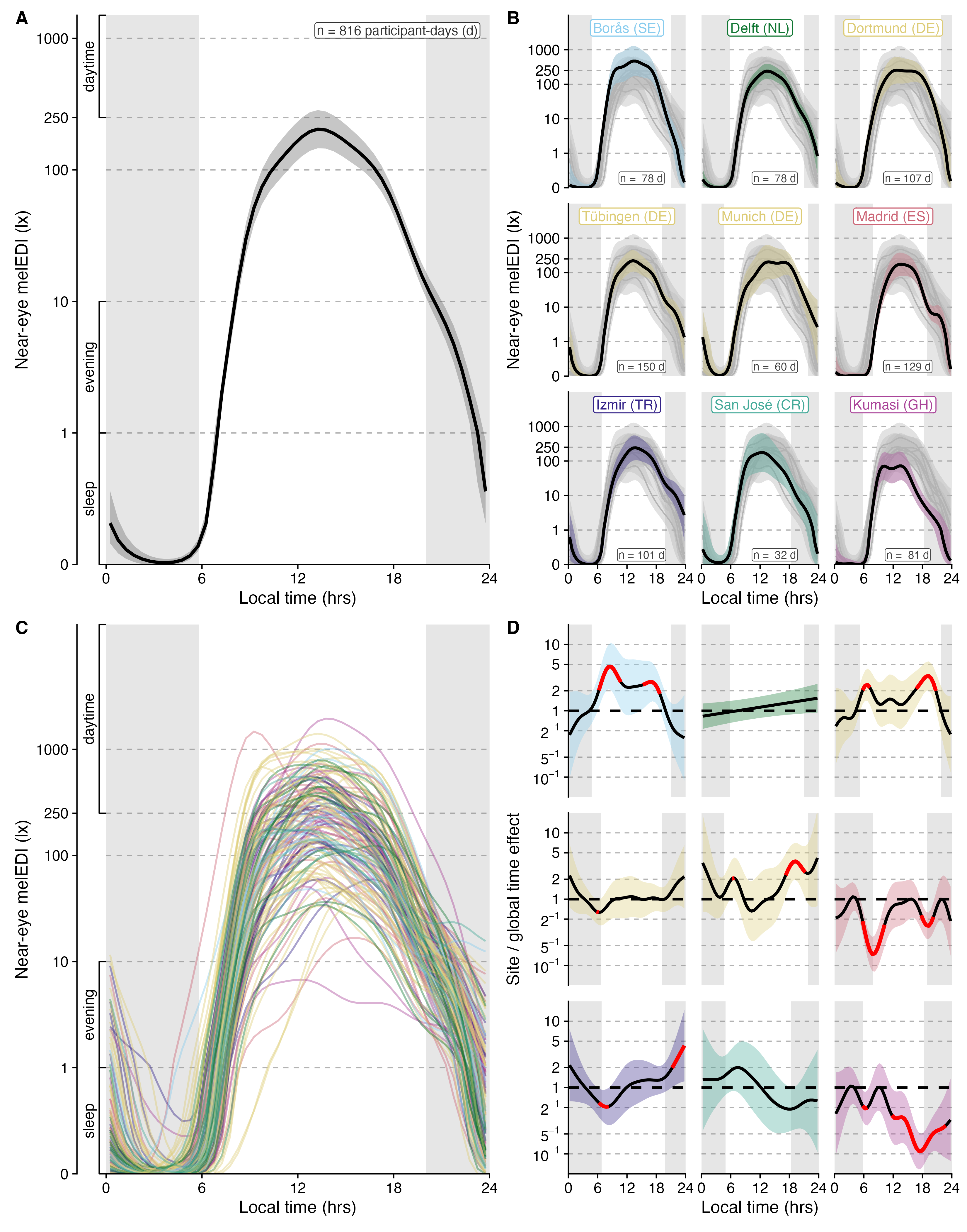
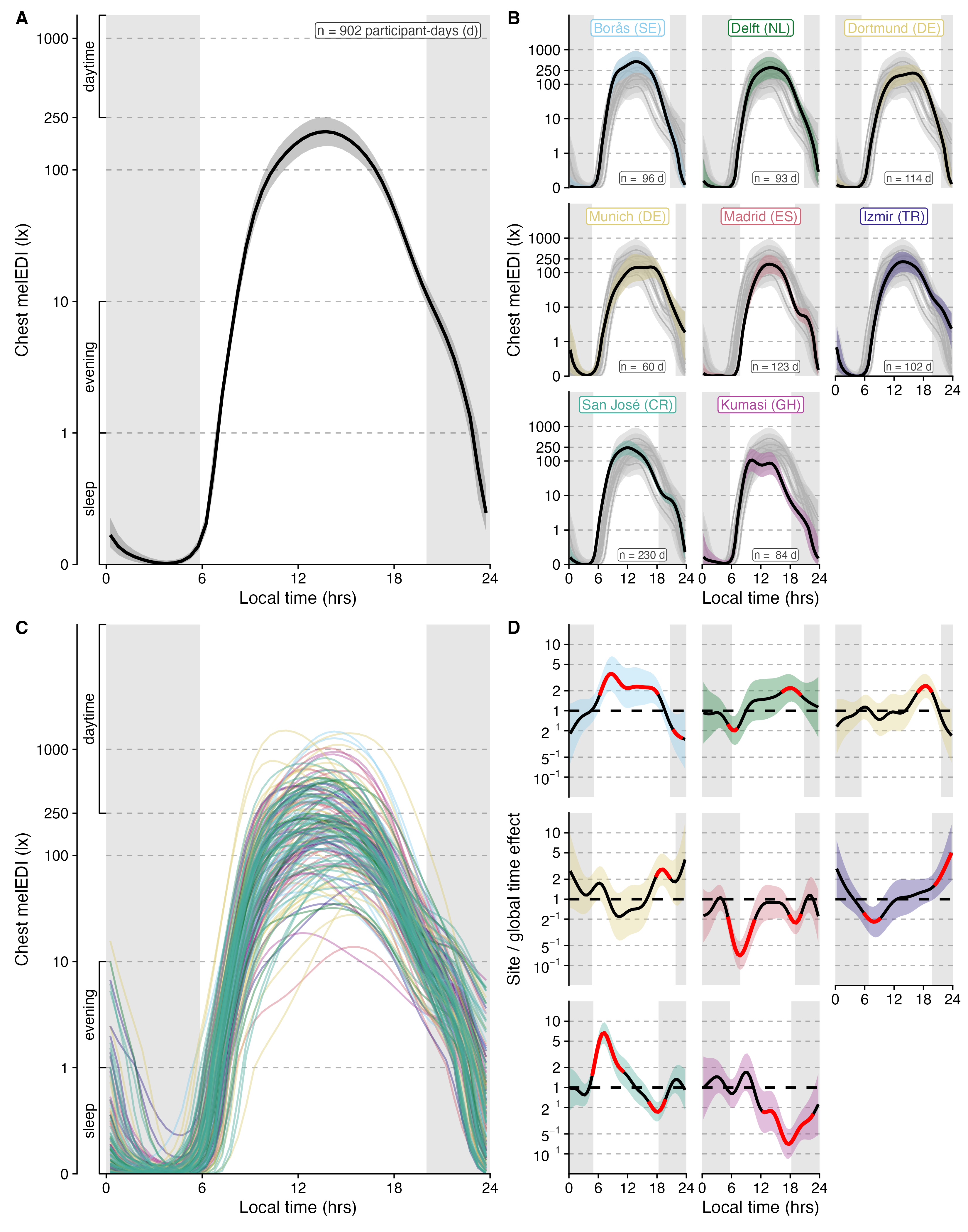
Calculate conditional pointwise intervals from the model covariance matrix, distinguish them from simultaneous intervals, and add civil-night context for the exact fitted participant-days. Both sensor positions use the same figure construction.
```{r}
#| label: h02-pointwise-figures
library(patchwork)
library(legendry)
library(ggtext)
source("scripts/Brown_bracket.R")
source("scripts/hypotheses/H02/h02_figure4_pointwise.R")
run_id <- "main__glasses__all_available"
chest_run_id <- "main__chest__all_available"
figure_directory <- file.path(paths$figures, "H02")
table_directory <- file.path(paths$tables, "H02")
source_directory <- file.path(paths$source_data, "H02")
site_registry <- readr::read_csv(file.path(root, "config/site_display_registry.csv"), show_col_types = FALSE) |> arrange(display_order)
frame_path <- file.path(
  paths$model_data,
  "H02",
  paste0(run_id, ".rds")
)
model_path <- file.path(
  paths$models,
  "H02",
  paste0(run_id, "__selected_model.rds")
)
prediction_path <- file.path(
  paths$source_data,
  "H02",
  "site_curve_predictions.csv"
)
contribution_path <- file.path(
  paths$source_data,
  "H02",
  paste0(run_id, "__fitted_contributions.rds")
)
base_path <- file.path(
  paths$model_data,
  "base",
  "metrics_glasses_30_minute_context.rds"
)
chest_frame_path <- file.path(
  paths$model_data,
  "H02",
  paste0(chest_run_id, ".rds")
)
chest_model_path <- file.path(
  paths$models,
  "H02",
  paste0(chest_run_id, "__selected_model.rds")
)
chest_contribution_path <- file.path(
  paths$source_data,
  "H02",
  paste0(chest_run_id, "__fitted_contributions.rds")
)
chest_base_path <- file.path(
  paths$model_data,
  "base",
  "metrics_chest_30_minute_context.rds"
)

near_eye_contract <- h02_build_figure_contract(
  run_id = run_id,
  placement_label = "Near-eye",
  frame_path = frame_path,
  model_path = model_path,
  contribution_path = contribution_path,
  base_path = base_path,
  prediction_path = prediction_path,
  site_registry = site_registry
)
chest_contract <- h02_build_figure_contract(
  run_id = chest_run_id,
  placement_label = "Chest",
  frame_path = chest_frame_path,
  model_path = chest_model_path,
  contribution_path = chest_contribution_path,
  base_path = chest_base_path,
  prediction_path = prediction_path,
  site_registry = site_registry
)
figure4 <- h02_build_figure4_layout(near_eye_contract)
figure4_chest <- h02_build_figure4_layout(chest_contract)
pointwise_windows <- h02_pointwise_windows(list(
  near_eye_contract,
  chest_contract
))


for (placement in c("near_eye", "chest")) {
  contract <- if (placement == "near_eye") near_eye_contract else chest_contract
  plot <- if (placement == "near_eye") figure4 else figure4_chest
  suffix <- if (placement == "near_eye") "" else "_chest"
  for (extension in c("png", "svg", "pdf")) {
    write_h02_plot(plot, file.path(figure_directory, paste0("daily_patterns", suffix, ".", extension)), width = 11, height = 14)
  }
  write_h02_rds(contract, file.path(source_directory, paste0("daily_patterns_source", suffix, ".rds")))
  for (name in names(contract)) {
    if (is.data.frame(contract[[name]])) {
      write_h02_csv(contract[[name]], file.path(source_directory, paste0("daily_patterns_", placement, "_", name, ".csv")))
    }
  }
}
write_h02_csv(pointwise_windows, file.path(table_directory, "figure4_pointwise_conditional_windows.csv"))
pointwise_windows |> head()
```
## Draw residual diagnostic figures
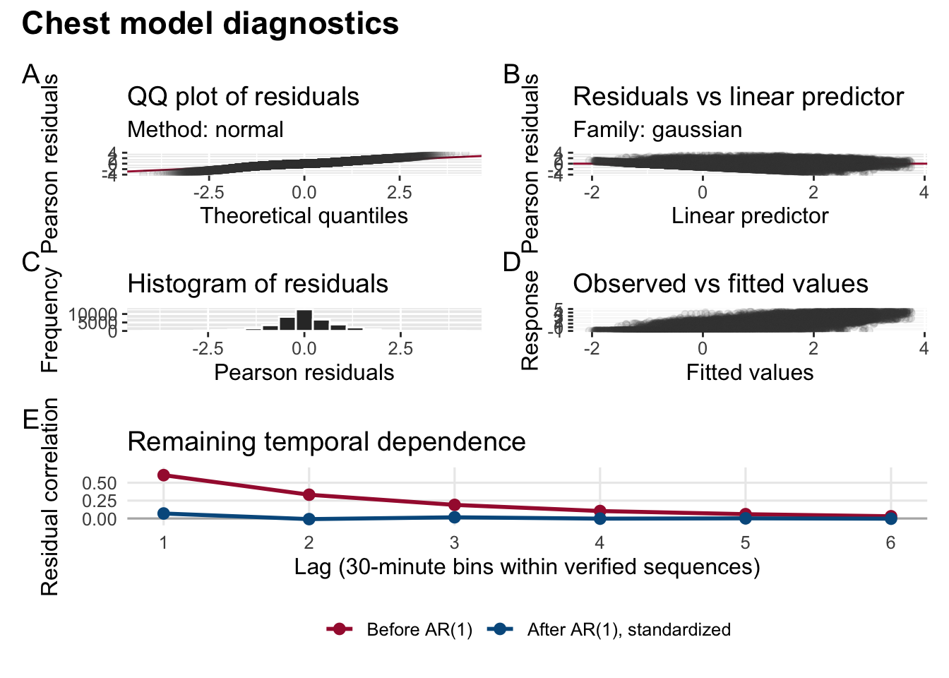
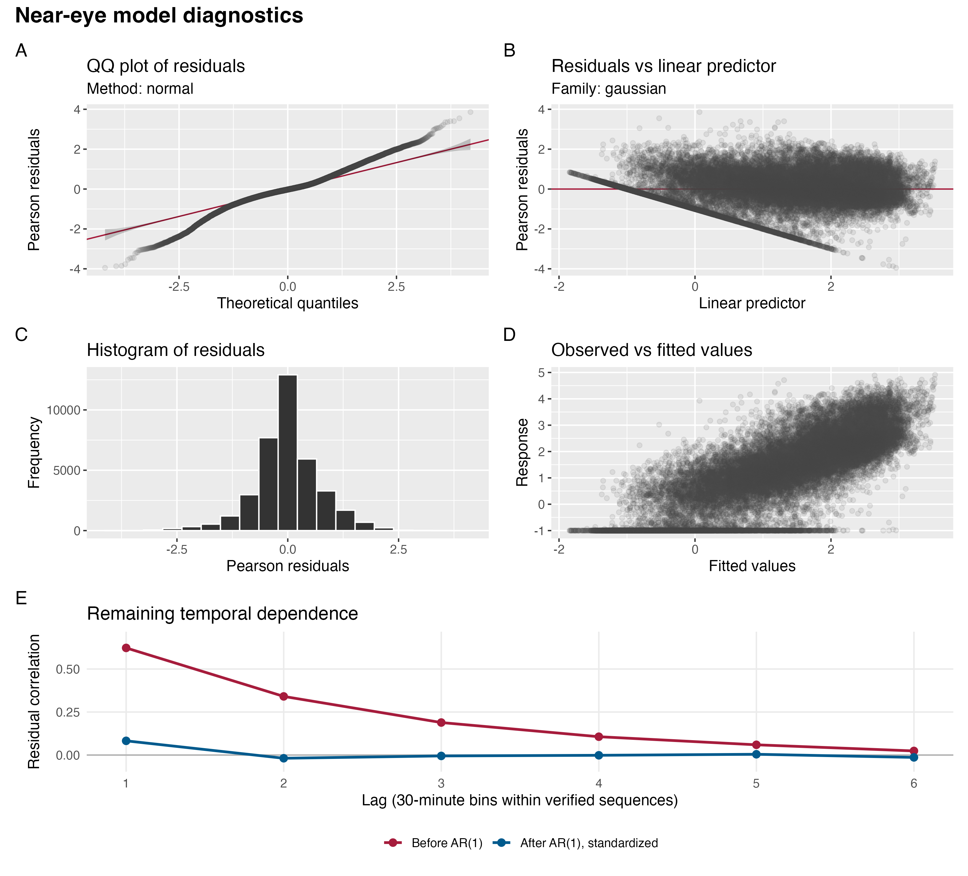
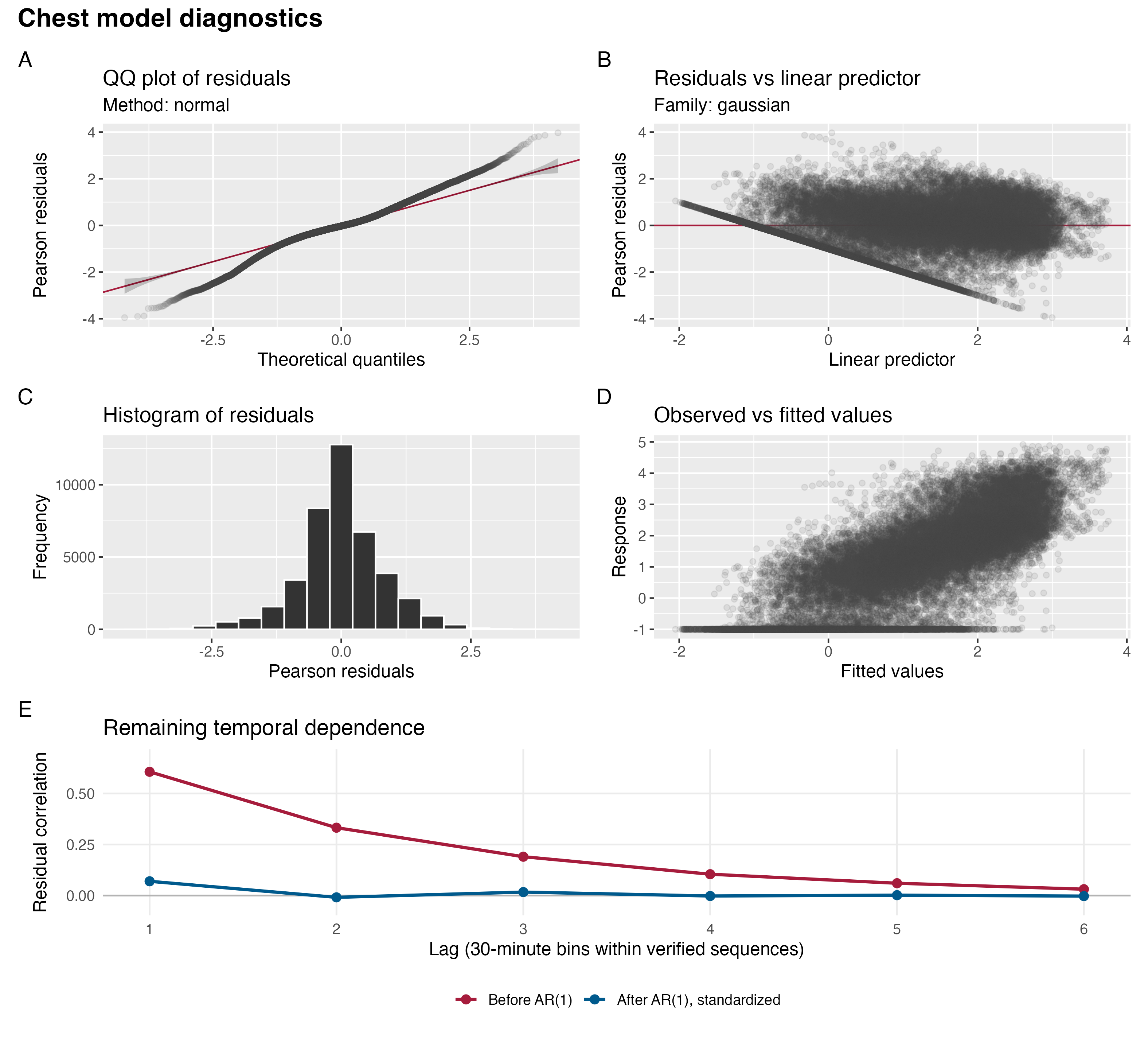
Display distributional diagnostics together with the within-sequence residual autocorrelation. Export the exact response, fitted values, residuals, and grouping fields behind the plots.
```{r}
#| label: h02-residual-figures
write_plot <- function(plot, path, width = 10.5, height = 9.5) {
  temporary <- tempfile(
    pattern = paste0(tools::file_path_sans_ext(basename(path)), "."),
    tmpdir = dirname(path),
    fileext = paste0(".", tools::file_ext(path))
  )
  on.exit(unlink(temporary), add = TRUE)
  ggplot2::ggsave(
    filename = temporary,
    plot = plot,
    width = width,
    height = height,
    units = "in",
    dpi = 300,
    bg = "white"
  )
  atomic_replace_artifact(temporary, path)
  invisible(path)
}

residual_acf <- readr::read_csv(
  file.path(root, "results", "csv/diagnostics", "H02", "residual_acf.csv"),
  show_col_types = FALSE
)

run_specification <- tibble::tribble(
  ~run_id, ~placement_label, ~file_stem,
  "main__glasses__all_available", "Near-eye", "near_eye",
  "main__chest__all_available", "Chest", "chest"
)

for (index in seq_len(nrow(run_specification))) {
  run_id <- run_specification$run_id[[index]]
  placement_label <- run_specification$placement_label[[index]]
  file_stem <- run_specification$file_stem[[index]]
  model_path <- file.path(
    root,
    "results", "models",
    "H02",
    paste0(run_id, "__selected_model.rds")
  )
  model <- readRDS(model_path)
  if (!inherits(model, "bam")) {
    stop(sprintf("Expected a bam object for %s", run_id), call. = FALSE)
  }
  if (length(model$std.rsd) != nrow(model$model)) {
    stop(sprintf("Residual/model-row mismatch for %s", run_id), call. = FALSE)
  }

  appraisal <- gratia::appraise(
    model,
    method = "normal",
    type = "pearson",
    ncol = 2,
    point_col = "grey25",
    point_alpha = 0.10,
    line_col = "#A61C3C"
  ) &
    ggplot2::theme(
      text = ggplot2::element_text(size = 12),
      plot.title = ggplot2::element_text(size = 14)
    )

  acf_data <- residual_acf |>
    dplyr::filter(.data$run_id == .env$run_id) |>
    dplyr::mutate(
      stage = factor(
        .data$stage,
        levels = c("preliminary_no_AR1", "final_AR1_standardized"),
        labels = c(
          "Before AR(1)",
          "After AR(1), standardized"
        )
      )
    )
  if (nrow(acf_data) != 12L) {
    stop(sprintf("Expected 12 residual-ACF rows for %s", run_id), call. = FALSE)
  }
  acf_plot <- ggplot2::ggplot(
    acf_data,
    ggplot2::aes(
      x = .data$lag_30_minute_bins,
      y = .data$correlation,
      colour = .data$stage,
      group = .data$stage
    )
  ) +
    ggplot2::geom_hline(yintercept = 0, colour = "grey70") +
    ggplot2::geom_line(linewidth = 1.0) +
    ggplot2::geom_point(size = 2.4) +
    ggplot2::scale_x_continuous(breaks = seq_len(6L)) +
    ggplot2::scale_colour_manual(
      values = c("Before AR(1)" = "#A61C3C", "After AR(1), standardized" = "#005A8D")
    ) +
    ggplot2::coord_cartesian(ylim = c(-0.06, 0.68)) +
    ggplot2::labs(
      x = "Lag (30-minute bins within verified sequences)",
      y = "Residual correlation",
      colour = NULL,
      title = "Remaining temporal dependence"
    ) +
    ggplot2::theme_minimal(base_size = 12) +
    ggplot2::theme(
      legend.position = "bottom",
      panel.grid.minor = ggplot2::element_blank()
    )

  diagnostic_figure <- (appraisal / acf_plot) +
    patchwork::plot_layout(heights = c(3.1, 1)) +
    patchwork::plot_annotation(
      title = paste(placement_label, "model diagnostics"),
      tag_levels = "A",
      theme = ggplot2::theme(
        plot.title = ggplot2::element_text(size = 17, face = "bold"),
        plot.tag = ggplot2::element_text(size = 15, face = "bold")
      )
    )

  png_path <- file.path(
    figure_directory,
    paste0("model_diagnostics_", file_stem, ".png")
  )
  pdf_path <- file.path(
    figure_directory,
    paste0("model_diagnostics_", file_stem, ".pdf")
  )
  write_plot(diagnostic_figure, png_path)
  write_plot(diagnostic_figure, pdf_path)

  plot_source <- tibble::tibble(
    run_id = run_id,
    response = model$model$response,
    linear_predictor = unname(model$linear.predictors),
    fitted_value = unname(model$fitted.values),
    pearson_residual = unname(stats::residuals(model, type = "pearson")),
    ar_standardized_residual = unname(model$std.rsd),
    site = as.character(model$model$site),
    participant = as.character(model$model$participant),
    participant_day = as.character(model$model$participant_day),
    time_hour = model$model$time_hour,
    ar_start = as.logical(model$model[["(AR.start)"]])
  )
  source_path <- file.path(
    source_directory,
    paste0("model_diagnostics_", file_stem, "_source.rds")
  )
  write_h02_csv(plot_source, sub("[.]rds$", ".csv", source_path))
  write_rds_artifact(
    plot_source,
    source_path,
    producer,
    list(
      run_id = run_id,
      residual_appraisal = "gratia::appraise(method = normal, type = pearson)",
      temporal_panel = "boundary-aware ACF from residual_acf.csv"
    )
  )

}
diagnostic_figure
```
## Compare sensor positions on matched observations
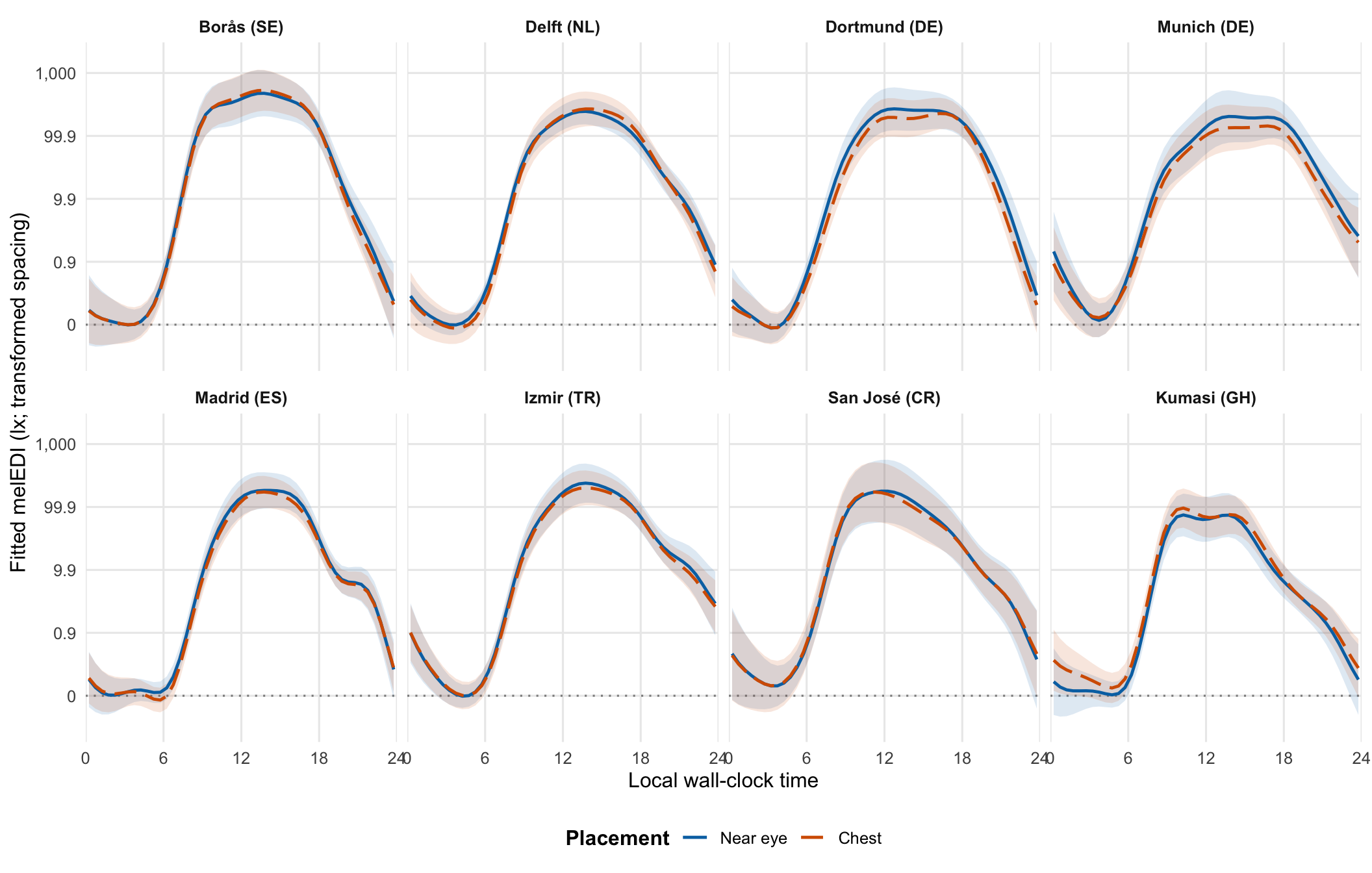
Require identical participant, day, and clock-bin keys before combining the near-eye and chest curve estimates. This comparison uses the common sample and does not treat the two sensor positions as interchangeable.
```{r}
#| label: h02-paired-placement
near_id <- "main__glasses__paired_common_sample"
chest_id <- "main__chest__paired_common_sample"

near_frame_path <- file.path(paths$model_data, "H02", paste0(near_id, ".rds"))
chest_frame_path <- file.path(
  paths$model_data,
  "H02",
  paste0(chest_id, ".rds")
)
prediction_path <- file.path(
  paths$source_data,
  "H02",
  "site_curve_predictions.csv"
)
sample_path <- file.path(paths$model_data, "H02", "sample_counts.csv")
registry_path <- file.path(root, "config", "site_display_registry.csv")
output_path <- file.path(
  paths$source_data,
  "H02",
  "paired_placement_site_curves.csv"
)

required_inputs <- c(
  near_frame_path,
  chest_frame_path,
  prediction_path,
  sample_path,
  registry_path
)
if (any(!file.exists(required_inputs))) {
  h02_abort(
    "Missing H02 paired-placement input(s): %s",
    paste(required_inputs[!file.exists(required_inputs)], collapse = ", ")
  )
}

near_frame <- readRDS(near_frame_path)
chest_frame <- readRDS(chest_frame_path)
observation_key <- c(
  "participant_key",
  "participant_day_key",
  "site",
  "clock_bin",
  "time_hour"
)
if (
  nrow(near_frame) != nrow(chest_frame) ||
    !identical(near_frame[observation_key], chest_frame[observation_key])
) {
  h02_abort("Near-eye and chest common-sample observation keys do not match")
}

sample_counts <- readr::read_csv(sample_path, show_col_types = FALSE)
paired_counts <- sample_counts |>
  dplyr::filter(
    .data$run_id %in% c(.env$near_id, .env$chest_id),
    .data$site == "ALL_SITES"
  ) |>
  dplyr::arrange(match(.data$run_id, c(.env$near_id, .env$chest_id)))
count_columns <- c(
  "participants",
  "participant_days",
  "observations_30_minute",
  "sites"
)
if (
  nrow(paired_counts) != 2L ||
    any(vapply(
      count_columns,
      function(column) {
        length(unique(paired_counts[[column]])) != 1L
      },
      logical(1)
    )) ||
    paired_counts$observations_30_minute[[1L]] != nrow(near_frame)
) {
  h02_abort("Recorded H02 paired-placement sample counts do not match")
}
if (!identical(
  unname(as.integer(paired_counts[1L, count_columns])),
  c(112L, 643L, 29786L, 8L)
)) {
  h02_abort("Unexpected H02 paired-placement sample identity")
}

site_registry <- readr::read_csv(registry_path, show_col_types = FALSE) |>
  dplyr::arrange(.data$display_order)
predictions <- readr::read_csv(prediction_path, show_col_types = FALSE) |>
  dplyr::filter(.data$run_id %in% c(.env$near_id, .env$chest_id))
curve_key <- c("site", "clock_bin", "time_hour")
near_keys <- predictions |>
  dplyr::filter(.data$run_id == .env$near_id) |>
  dplyr::select(dplyr::all_of(curve_key))
chest_keys <- predictions |>
  dplyr::filter(.data$run_id == .env$chest_id) |>
  dplyr::select(dplyr::all_of(curve_key))
if (
  nrow(near_keys) != 384L ||
    !identical(near_keys, chest_keys) ||
    anyDuplicated(near_keys)
) {
  h02_abort("Stored paired-placement site-curve grids do not match")
}

critical <- stats::qnorm(0.975)
paired_sample <- paired_counts[1L, count_columns]
display_data <- predictions |>
  dplyr::mutate(
    placement = dplyr::recode(
      .data$run_id,
      !!near_id := "Near eye",
      !!chest_id := "Chest"
    ),
    pointwise_lower_eta = .data$eta - critical * .data$standard_error,
    pointwise_upper_eta = .data$eta + critical * .data$standard_error,
    pointwise_lower_melEDI_lx = h02_inverse_transform(
      .data$pointwise_lower_eta
    ),
    pointwise_upper_melEDI_lx = h02_inverse_transform(
      .data$pointwise_upper_eta
    )
  ) |>
  dplyr::left_join(
    site_registry,
    by = "site",
    relationship = "many-to-one"
  ) |>
  dplyr::mutate(
    paired_participants = paired_sample$participants,
    paired_participant_days = paired_sample$participant_days,
    paired_observations_30_minute = paired_sample$observations_30_minute,
    paired_sites = paired_sample$sites,
    placement_order = match(.data$placement, c("Near eye", "Chest"))
  ) |>
  dplyr::arrange(
    .data$display_order,
    .data$clock_bin,
    .data$placement_order
  ) |>
  dplyr::select(
    "run_id",
    "placement",
    "site",
    "display_name",
    "display_order",
    "color_hex",
    "clock_bin",
    "time_hour",
    "eta",
    "standard_error",
    "pointwise_lower_eta",
    "pointwise_upper_eta",
    "estimate_melEDI_lx",
    "pointwise_lower_melEDI_lx",
    "pointwise_upper_melEDI_lx",
    "paired_participants",
    "paired_participant_days",
    "paired_observations_30_minute",
    "paired_sites"
  )

if (
  nrow(display_data) != 768L ||
    anyNA(display_data[c("display_name", "display_order", "color_hex")]) ||
    any(display_data$pointwise_lower_eta > display_data$eta) ||
    any(display_data$pointwise_upper_eta < display_data$eta)
) {
  h02_abort("Invalid H02 paired-placement display data")
}

invisible(write_csv_artifact(display_data, output_path, producer))
display_data |> head()
```
## Bind the displayed results to the estimates
The following extracts select the primary, complementary, and sensitivity estimates for the tables and accompanying interpretation.
```{r}
#| label: h02-reader-bindings
source("scripts/hypotheses/H02/h02_reader_helpers.R")
suppressPackageStartupMessages({
  library(dplyr)
  library(ggplot2)
  library(gt)
  library(readr)
  library(tibble)
  library(tidyr)
})

root <- normalizePath(
  Sys.getenv("QUARTO_PROJECT_DIR", unset = getwd()),
  winslash = "/",
  mustWork = TRUE
)

source(file.path(root, "scripts", "pipeline", "p_value_display.R"))

site_registry <- read_h02_csv("config", "site_display_registry.csv") |>
  arrange(.data$display_order)

sample_counts <- read_h02_csv(
  "results", "intermediate/model_data", "H02", "sample_counts.csv"
)

support_audit <- read_h02_csv(
  "results", "intermediate/model_data", "H02", "support_audit.csv"
)

model_fits <- read_h02_csv(
  "results", "tables", "H02", "model_fit_summary.csv"
)

model_comparisons <- read_h02_csv(
  "results", "tables", "H02", "model_structure_comparisons.csv"
)

variation <- read_h02_csv(
  "results", "tables", "H02", "variation_summary.csv"
)

dominance <- read_h02_csv(
  "results", "tables", "H02", "dominance_summary.csv"
)

dominance_comparison <- read_h02_csv(
  "results", "tables", "H02", "dominance_comparison_summary.csv"
)

pointwise_windows <- read_h02_csv(
  "results", "tables", "H02",
  "figure4_pointwise_conditional_windows.csv"
)

residual_acf <- read_h02_csv(
  "results", "csv/diagnostics", "H02", "residual_acf.csv"
)

residual_summary <- read_h02_csv(
  "results", "csv/diagnostics", "H02", "residual_summary.csv"
)

cluster_acf <- read_h02_csv(
  "results", "csv/diagnostics", "H02",
  "cluster_residual_acf_summary.csv"
)

k_checks <- read_h02_csv(
  "results", "csv/diagnostics", "H02",
  "basis_dimension_checks.csv"
)

sz_checks <- read_h02_csv(
  "results", "csv/diagnostics", "H02",
  "sz_constraint_identifiability.csv"
)

concurvity <- read_h02_csv(
  "results", "csv/diagnostics", "H02", "formal_concurvity.csv"
)

preparation_sensitivity <- read_h02_csv(
  "results", "tables", "H02",
  "alternative_preprocessing_stability.csv"
)

formula_sensitivity <- read_h02_csv(
  "results", "tables", "H02",
  "formula_sensitivity_comparison.csv"
)

paired_placement_curves <- read_h02_csv(
  "results", "csv/source_data", "H02",
  "paired_placement_site_curves.csv"
)

near_id <- "main__glasses__all_available"

chest_id <- "main__chest__all_available"

paired_near_id <- "main__glasses__paired_common_sample"

paired_chest_id <- "main__chest__paired_common_sample"

alternative_preparation_id <-
  "alternative_preprocessing__glasses__all_available"

near_counts <- sample_overall(near_id)

chest_counts <- sample_overall(chest_id)

near_variation <- variation |>
  filter(.data$run_id == near_id)

chest_variation <- variation |>
  filter(.data$run_id == chest_id)

near_dominance <- dominance |>
  filter(.data$run_id == near_id)

chest_dominance <- dominance |>
  filter(.data$run_id == chest_id)

near_dominance_comparison <- dominance_comparison |>
  filter(.data$run_id == near_id)

chest_dominance_comparison <- dominance_comparison |>
  filter(.data$run_id == chest_id)

site_test <- model_comparisons |>
  filter(.data$comparison_id == "site_pattern_vs_no_site")

deviations_model <- tibble::tribble(
  ~Aspect, ~Registered, ~Analysis, ~Reason_or_consequence,
  "Primary placement",
  "Chest primary; near-eye repeat",
  "Near-eye primary; chest complementary",
  "Near-eye better represents light close to the eye; placements are not pooled.",
  "Outcome and epoch",
  "Hourly geometric-mean melEDI",
  "30-minute arithmetic-mean melEDI",
  "Provides clock-resolved support but changes the outcome and dependence structure.",
  "Response scale",
  "No zero-handling transform specified",
  "log10(melEDI + 0.1 lx)",
  "Retains exact zero observations while defining a finite modelling scale.",
  "Global time effect",
  "No separate overall smooth",
  "Cyclic global time smooth, k = 12",
  "Makes site curves deviations from one shared daily profile.",
  "Site smooth",
  "Site-specific cyclic cc smooths",
  "Sum-to-zero sz deviations, k = 12; default time marginal is not cyclic",
  "Sum-to-zero site contrasts replace reference-site comparisons.",
  "Participant hierarchy",
  "Participant-time factor smooth",
  "Participant factor smooth (k = 10) plus participant-day random intercept",
  "Separates person-specific shape from day-to-day level shifts.",
  "Variance target",
  "Within-participant variance exceeds between-site variance",
  "Integrated fitted-curve dispersion plus conditional Shapley allocation",
  "The reported quantities are explicitly defined and are not response variance explained."
)

deviations_data <- tibble::tribble(
  ~Aspect, ~Registered_or_unspecified, ~Analysis, ~Reason_or_consequence,
  "30-minute support",
  "Hourly outcome; no 30-minute rule",
  "At least 15 valid one-minute values per 30-minute bin",
  "Unsupported bins remain missing rather than being treated as darkness.",
  "Whole-day handling",
  "Coverage-based exclusion; no exact-zero-day rule",
  "No additional daily-coverage deletion for H02; entirely exact-zero days are excluded",
  "Preserves partly observed days while removing the fixed signal-plausibility failure.",
  "Clock and DST",
  "Not operationally specified",
  "Local wall clock for profiles; true UTC for ordering; fall-back folds retained",
  "AR sequences reset at every participant-day and discontinuity.",
  "Measurement context",
  "Wear and sleep removal described generally",
  "Wake values are worn measurements; sleep values describe the bedside environment",
  "The 24-hour record is hybrid and is not continuous ocular exposure.",
  "Operating range",
  "Values above 120,000 lx excluded",
  "melEDI must be below 100,000 lx after one-minute aggregation",
  "Uses the manufacturer operating boundary."
)

primary_ratios <- bind_rows(
  ratio_row(near_id, "participant_to_site_ratio") |>
    mutate(Scenario = "Primary near-eye"),
  ratio_row(near_id, "participant_plus_day_to_site_ratio") |>
    mutate(Scenario = "Primary near-eye")
)

alternative_counts <- sample_overall(alternative_preparation_id)

paired_near_counts <- sample_overall(paired_near_id)

paired_chest_counts <- sample_overall(paired_chest_id)

near_participant_ratio <- extract_ratio(
  near_id, "participant_to_site_ratio"
)
near_combined_ratio <- extract_ratio(
  near_id, "participant_plus_day_to_site_ratio"
)

alternative_participant_ratio <- extract_ratio(
  alternative_preparation_id, "participant_to_site_ratio"
)

alternative_combined_ratio <- extract_ratio(
  alternative_preparation_id, "participant_plus_day_to_site_ratio"
)

paired_near_participant_ratio <- extract_ratio(
  paired_near_id, "participant_to_site_ratio"
)

paired_near_combined_ratio <- extract_ratio(
  paired_near_id, "participant_plus_day_to_site_ratio"
)

chest_participant_ratio <- extract_ratio(
  chest_id, "participant_to_site_ratio"
)

chest_combined_ratio <- extract_ratio(
  chest_id, "participant_plus_day_to_site_ratio"
)

paired_chest_participant_ratio <- extract_ratio(
  paired_chest_id, "participant_to_site_ratio"
)

paired_chest_combined_ratio <- extract_ratio(
  paired_chest_id, "participant_plus_day_to_site_ratio"
)

cyclic_participant_ratio <- formula_sensitivity |>
  filter(
    .data$data_scenario_id == "main",
    .data$summary_id == "participant_to_site_ratio"
  )

cyclic_combined_ratio <- formula_sensitivity |>
  filter(
    .data$data_scenario_id == "main",
    .data$summary_id == "participant_plus_day_to_site_ratio"
  )

sensitivity_display <- bind_rows(
  make_sensitivity_row(
    "Primary near-eye",
    near_counts$participants,
    near_counts$participant_days,
    near_counts$observations_30_minute,
    near_participant_ratio$estimate,
    near_participant_ratio$lower_95,
    near_participant_ratio$upper_95,
    near_combined_ratio$estimate,
    near_combined_ratio$lower_95,
    near_combined_ratio$upper_95,
    "Reference result"
  ),
  make_sensitivity_row(
    "Gap-timing-unaware dataset",
    alternative_counts$participants,
    alternative_counts$participant_days,
    alternative_counts$observations_30_minute,
    alternative_participant_ratio$estimate,
    alternative_participant_ratio$lower_95,
    alternative_participant_ratio$upper_95,
    alternative_combined_ratio$estimate,
    alternative_combined_ratio$lower_95,
    alternative_combined_ratio$upper_95,
    "Stable"
  ),
  make_sensitivity_row(
    "Cyclic site and participant deviations",
    near_counts$participants,
    near_counts$participant_days,
    near_counts$observations_30_minute,
    cyclic_participant_ratio$cyclic_sensitivity_estimate,
    cyclic_participant_ratio$cyclic_sensitivity_lower_95,
    cyclic_participant_ratio$cyclic_sensitivity_upper_95,
    cyclic_combined_ratio$cyclic_sensitivity_estimate,
    cyclic_combined_ratio$cyclic_sensitivity_lower_95,
    cyclic_combined_ratio$cyclic_sensitivity_upper_95,
    "Stable"
  ),
  make_sensitivity_row(
    "Placement-matched near eye",
    paired_near_counts$participants,
    paired_near_counts$participant_days,
    paired_near_counts$observations_30_minute,
    paired_near_participant_ratio$estimate,
    paired_near_participant_ratio$lower_95,
    paired_near_participant_ratio$upper_95,
    paired_near_combined_ratio$estimate,
    paired_near_combined_ratio$lower_95,
    paired_near_combined_ratio$upper_95,
    "Combined ordering retained; participant-only interval includes 1"
  ),
  make_sensitivity_row(
    "Complementary chest",
    chest_counts$participants,
    chest_counts$participant_days,
    chest_counts$observations_30_minute,
    chest_participant_ratio$estimate,
    chest_participant_ratio$lower_95,
    chest_participant_ratio$upper_95,
    chest_combined_ratio$estimate,
    chest_combined_ratio$lower_95,
    chest_combined_ratio$upper_95,
    "Combined ordering retained; participant-only interval includes 1"
  ),
  make_sensitivity_row(
    "Placement-matched chest",
    paired_chest_counts$participants,
    paired_chest_counts$participant_days,
    paired_chest_counts$observations_30_minute,
    paired_chest_participant_ratio$estimate,
    paired_chest_participant_ratio$lower_95,
    paired_chest_participant_ratio$upper_95,
    paired_chest_combined_ratio$estimate,
    paired_chest_combined_ratio$lower_95,
    paired_chest_combined_ratio$upper_95,
    "Combined ordering retained; participant-only interval includes 1"
  )
)
```
## Question {#findings}
The preregistered hypothesis was:
> “Within-participant variance in hourly melanopic EDI, with participants
> nested in sites, exceeds variance between sites.”
The preregistered model was:
```r
Metric ~ Site +
  s(Time, by = Site, bs = "cc", k = 12) +
  s(Participant, Time, bs = "fs")
```
The scientific question is whether daily patterns of **melanopic equivalent
daylight illuminance (melEDI)** differ among sites, how much people within a
site differ from one another, and whether those within-site differences are
larger than the differences among sites.
::: {.callout-note title="Answer in brief"}
Near-eye daily patterns differed among sites
($\chi^2=$ `r fmt_number(site_test$test_statistic, 2)`,
`r fmt_number(site_test$test_df, 0)` degrees of freedom,
false-discovery-rate (FDR)-adjusted $p$ = `r fmt_p_value(site_test$p_adjusted, site_test$p_adjusted < 0.05)`).
Participant curves plus participant-day shifts were
`r fmt_ci(near_combined_ratio$estimate, near_combined_ratio$lower_95, near_combined_ratio$upper_95, 2)`
times as dispersed as site curves. In the conditional Shapley analysis, those
two participant-level blocks received
`r with(filter(near_dominance_comparison, comparison_id == "participant_plus_day_to_site_shapley_ratio"), fmt_ci(estimate, lower_95, upper_95, 2))`
times as much in-sample model-fit credit as the site-pattern block. Chest
measurements gave the same combined ordering.
:::
## What was analysed
The near-eye sensor position is primary because it measures light closer to the
eye, but it is not a direct retinal measurement. The chest sensor position is
analysed separately as complementary evidence and is not a measure of ocular
exposure; the two placements are never pooled. During reported sleep, both
positions characterize the bedside light environment rather than light at
their nominal worn position.
A **participant-day** is one participant's observations on one local calendar
date. Counts of participant-days therefore describe repeated recorded days,
not additional independent participants.
The model used local wall-clock time to describe the daily pattern. True UTC
time determined observation ordering. A 30-minute bin entered the model when
at least 15 of its 30 one-minute melEDI values were valid. Missing, unsupported,
non-wear, and out-of-range values remained missing, not zero. Repeated
fall-back clock bins retained their fold provenance; residual sequences were
reset at each participant-day, after any elapsed-time discontinuity, and
around a wall-clock outcome without a one-to-one true-time coordinate.
### Terms used below
- A **nonlinear GAM analysis** uses a generalized additive model (GAM), which
allows the association with local clock time to bend across the day rather
than forcing it to follow a straight line.
- The model uses `log10(melEDI + 0.1 lx)`. A **back-transformed** curve applies
the inverse transformation and returns to melEDI in lux.
- Participant and participant-day smooths represent fitted variation that
remains among people or recorded days after the time and site patterns have
been considered.
- **Autocorrelation** means adjacent 30-minute residuals can remain more alike
than residuals farther apart. The AR(1) structure represents this dependence
as strongest for adjacent observations and weaker at longer lags.
- A **pointwise 95% confidence interval (95% CI)** gives uncertainty at one
displayed clock time. It is not a simultaneous band for the full day and
does not multiplicity-control every red segment in a daily curve.
- **Shapley allocation** averages a model component's contribution over all
orders in which components could be added, allocating shared fitted-model
information rather than counting it repeatedly.
The complete [registration-change record](#h02-preregistration-deviations)
appears in the detailed analysis record.
## Model
The daily patterns were estimated with a nonlinear GAM analysis. This model
combines a curved time-of-day pattern with structured departures for sites,
participants, and participant-days while retaining the repeated-measures
structure.
The exact Wilkinson formula was:
```r
response ~
  s(time_hour, bs = "cc", k = 12) +
  s(time_hour, site, bs = "sz", k = 12) +
  s(time_hour, participant, bs = "fs", k = 10) +
  s(participant_day, bs = "re")
```
Here, `response` is
$\log_{10}(\mathrm{melEDI}+0.1\ \mathrm{lx})$.
The first term is the **global time effect**, which is the site-average daily
curve: it gives every site equal weight and joins smoothly at midnight. The
`sz` term estimates how each site's curve departs from that site-average curve;
the departures sum to zero, so no reference site is required. The participant
smooth represents remaining differences in daily shape among people after the
reported time and site patterns are considered. Participant identifiers are
site-prefixed, so people remain nested within sites. The participant-day random
effect represents remaining day-to-day level shifts within participants after
those patterns are considered; it shifts an entire fitted day up or down
without changing its shape.
Only the global time effect is explicitly cyclic. The default time marginals
inside the `sz` site term and `fs` participant term are not forced to meet
at midnight. A fully cyclic formulation is therefore included as a
model-form sensitivity.
Because adjacent 30-minute residuals can remain more similar than residuals
farther apart, the model was fitted with `mgcv::bam()` under fREML and a
boundary-aware AR(1) working correlation. Site curves and their pointwise 95%
CIs were obtained from the fitted linear-predictor matrix and full coefficient
covariance. Each interval describes uncertainty at one clock time; it is not a
simultaneous band across the day. Smoothing parameters are treated as fixed in
these intervals. `gratia` was used for residual appraisal and for the
concurvity model check; concurvity is overlap among nonlinear model terms that
makes their separate contributions harder to distinguish.
### Quantities used to compare sites and people
The first comparison describes the spread of the fitted curves. On a common
48-bin clock grid,
$$
V_{\mathrm{site}} =
\frac{1}{48}\sum_b
\operatorname{Var}_{s}\{\hat f_s(t_b)\},
$$
and participant-curve variation is the within-site variance among participant
curves over the same clock grid, averaged across sites with each site receiving
equal weight. Participant-day variation uses the same site-average weighting
for the variance of day-specific intercept contributions. Their ratios compare
fitted curve dispersion on the transformed modelling scale. They are not
proportions of response variance and are not “variance explained.”
The second comparison asks which model block contributes more to in-sample
fit. The global time effect is retained in every model. Site pattern,
participant pattern, and participant-day shift are then included in every
possible combination. For each block, the conditional Shapley allocation is
its average increase in row-weighted in-sample $R^2$ across all possible
orders of entry. This allocates shared fitted-model information without
counting it repeatedly. It describes conditional in-sample model-fit relevance,
not causal importance or cross-validated predictive importance.
Both sets of 95% confidence intervals use `r format(bootstrap_count(2000L), big.mark = ",")` hierarchical cluster
resamples: sites, participants within sampled sites, and participant-days
within sampled participants. The fitted curve contributions or fitted subset
models are held fixed. The intervals therefore describe cluster-sampling
uncertainty conditional on the fitted smoothing structure.
## Primary near-eye result
The primary model fitted `r near_counts$participants` participants,
`r near_counts$participant_days` participant-days,
`r format(near_counts$observations_30_minute, big.mark = ",")` 30-minute
observations, and `r near_counts$sites` sites.
### Daily profiles
Panel A shows the global time effect, the site-average curve that gives each
site equal weight. Panel B shows the absolute fitted curve for each site; each
facet states its fitted participant-day count. Panel C overlays the fitted
participant curves. Panel D shows each site's fitted curve divided by the
global time effect. A factor of 2 means twice the fitted
$\mathrm{melEDI}+0.1\ \mathrm{lx}$ quantity; a factor of 0.5 means half. Grey
vertical bands show the mean civil-night intervals.
Ribbons in panels A, B, and D are pointwise 95% CIs. Red segments in panel D
identify individual 30-minute bins whose interval excludes one. These segments
are local descriptions, not jointly multiplicity-controlled tests across the
day or across sites.
```{r}
#| label: fig-h02-near-patterns
#| fig-cap: "Daily near-eye melEDI patterns: site-average curve (A), site curves (B), participant curves (C), and site-to-global-time-effect factors (D). Ribbons are pointwise 95% CIs."
#| fig-alt: "Four-panel near-eye daily-pattern figure. Panel A shows the site-average global time effect for 816 participant-days with a pointwise 95% confidence ribbon. Panel B shows nine site curves, pointwise ribbons, country-coded site labels, and a participant-day count in each facet. Panel C shows participant curves. Panel D shows site-to-global-time-effect factors with pointwise ribbons; red segments mark individual clock times whose intervals exclude one."
#| out-width: "88%"
#| fig-align: center
include_project_graphics(file.path(
  root,
  "results", "images",
  "H02",
  "daily_patterns.png"
))
```
### Fitted-curve dispersion
```{r}
#| label: tbl-h02-near-variation
#| tbl-cap: "Near-eye fitted-curve variation and participant-to-site ratios."
variation_table_data(near_id) |>
  gt::gt(rowname_col = "Quantity", groupname_col = "Section") |>
  gt::cols_align(align = "right", columns = c(Estimate, `95% CI`)) |>
  gt::tab_source_note(
    source_note = paste(
      "Variation units are squared log10(melEDI + 0.1 lx) prediction",
      "units. Participant / site divides participant-curve variation by",
      "site-curve variation; (Participant + day) / site adds participant-day",
      "intercept variation to that numerator. Ratios are unitless. CIs use",
      paste0(format(bootstrap_count(2000L), big.mark = ","), " hierarchical resamples.")
    )
  ) |>
  h02_gt()
```
Participant curves were
`r fmt_ci(near_participant_ratio$estimate, near_participant_ratio$lower_95, near_participant_ratio$upper_95, 2)`
times as dispersed as site curves. Adding participant-day shifts increased
that ratio to
`r fmt_ci(near_combined_ratio$estimate, near_combined_ratio$lower_95, near_combined_ratio$upper_95, 2)`.
Thus, fitted variation within sites was larger than fitted variation among
sites under the predeclared clock-grid definition.
### Relative contribution to fitted-model performance
```{r}
#| label: tbl-h02-near-dominance
#| tbl-cap: "Near-eye conditional Shapley allocation of in-sample model fit."
dominance_table_data(near_id) |>
  gt::gt(rowname_col = "Component") |>
  gt::tab_source_note(
    source_note = paste(
      "Full-model in-sample R² =",
      fmt_ci(
        near_dominance$full_model_R2[[1L]],
        near_dominance$full_model_R2_lower_95[[1L]],
        near_dominance$full_model_R2_upper_95[[1L]],
        3
      ),
      "."
    )
  ) |>
  h02_gt()
```
```{r}
#| label: tbl-h02-near-relevance
#| tbl-cap: "Near-eye participant-versus-site comparisons from the Shapley allocation."
dominance_comparison_data(near_id) |>
  gt::gt(rowname_col = "Comparison") |>
  gt::cols_align(align = "right", columns = Result) |>
  h02_gt()
```
Participant-specific patterns received
`r with(filter(near_dominance_comparison, comparison_id == "participant_to_site_shapley_ratio"), fmt_ci(estimate, lower_95, upper_95, 2))`
times as much in-sample model-fit credit as site patterns. Participant
patterns and participant-day shifts together received
`r with(filter(near_dominance_comparison, comparison_id == "participant_plus_day_to_site_shapley_ratio"), fmt_ci(estimate, lower_95, upper_95, 2))`
times as much credit as site patterns and accounted for
`r with(filter(near_dominance_comparison, comparison_id == "participant_plus_day_share_of_heterogeneity"), fmt_percent_ci(estimate, lower_95, upper_95, 1))`
of the fitted $R^2$ increment beyond the global time effect.
This is the most direct answer to “how much more relevant were participants
within sites than sites themselves”: in this fitted sample and model,
participant-level blocks contributed substantially more to in-sample fit than
the site-pattern block. It does not imply that changing a person's behaviour
would cause that amount of change.
### Pointwise site windows
```{r}
#| label: tbl-h02-near-windows
#| tbl-cap: "Near-eye clock windows whose pointwise conditional 95% interval excludes the global time effect."
window_table_data(near_id) |>
  gt::gt(rowname_col = "Site") |>
  gt::tab_source_note(
    source_note = paste(
      "Factors compare each site with the global time effect.",
      "The windows are not simultaneous curve-level discoveries."
    )
  ) |>
  h02_gt()
```
## Complementary chest result
The chest model used the identical formula, transform, fitting algorithm,
curve definitions, and interval procedures. It fitted
`r chest_counts$participants` participants,
`r chest_counts$participant_days` participant-days,
`r format(chest_counts$observations_30_minute, big.mark = ",")` 30-minute
observations, and `r chest_counts$sites` sites. Tübingen (DE) is absent because
chest measurements were unavailable there.
### Fitted-curve dispersion
```{r}
#| label: tbl-h02-chest-variation
#| tbl-cap: "Chest fitted-curve variation and participant-to-site ratios."
variation_table_data(chest_id) |>
  gt::gt(rowname_col = "Quantity", groupname_col = "Section") |>
  gt::cols_align(align = "right", columns = c(Estimate, `95% CI`)) |>
  gt::tab_source_note(
    source_note = paste(
      "Variation units are squared log10(melEDI + 0.1 lx) prediction",
      "units. Participant / site divides participant-curve variation by",
      "site-curve variation; (Participant + day) / site adds participant-day",
      "intercept variation to that numerator. Ratios are unitless. CIs use",
      paste0(format(bootstrap_count(2000L), big.mark = ","), " hierarchical resamples.")
    )
  ) |>
  h02_gt()
```
Chest participant curves were
`r fmt_ci(chest_participant_ratio$estimate, chest_participant_ratio$lower_95, chest_participant_ratio$upper_95, 2)`
times as dispersed as chest site curves. That interval includes one. After
participant-day shifts were included, the ratio was
`r fmt_ci(chest_combined_ratio$estimate, chest_combined_ratio$lower_95, chest_combined_ratio$upper_95, 2)`,
retaining the combined participant-level ordering.
### Relative contribution to fitted-model performance
```{r}
#| label: tbl-h02-chest-dominance
#| tbl-cap: "Chest conditional Shapley allocation of in-sample model fit."
dominance_table_data(chest_id) |>
  gt::gt(rowname_col = "Component") |>
  gt::tab_source_note(
    source_note = paste(
      "Full-model in-sample R² =",
      fmt_ci(
        chest_dominance$full_model_R2[[1L]],
        chest_dominance$full_model_R2_lower_95[[1L]],
        chest_dominance$full_model_R2_upper_95[[1L]],
        3
      ),
      "."
    )
  ) |>
  h02_gt()
```
```{r}
#| label: tbl-h02-chest-relevance
#| tbl-cap: "Chest participant-versus-site comparisons from the Shapley allocation."
dominance_comparison_data(chest_id) |>
  gt::gt(rowname_col = "Comparison") |>
  gt::cols_align(align = "right", columns = Result) |>
  h02_gt()
```
At the chest, participant patterns received
`r with(filter(chest_dominance_comparison, comparison_id == "participant_to_site_shapley_ratio"), fmt_ci(estimate, lower_95, upper_95, 2))`
times as much in-sample model-fit credit as site patterns. Participant
patterns plus participant-day shifts received
`r with(filter(chest_dominance_comparison, comparison_id == "participant_plus_day_to_site_shapley_ratio"), fmt_ci(estimate, lower_95, upper_95, 2))`
times as much credit. The complementary placement therefore reproduces the
relative-relevance ordering.
### Daily profiles
As in the near-eye figure, panel A shows the site-average global time effect,
panel B shows site curves with fitted participant-day counts, panel C shows
participant curves, and panel D shows site-to-global-time-effect factors.
Ribbons in panels A, B, and D are pointwise 95% CIs.
```{r}
#| label: fig-h02-chest-patterns
#| fig-cap: "Daily chest melEDI patterns: site-average curve (A), site curves (B), participant curves (C), and site-to-global-time-effect factors (D). Ribbons are pointwise 95% CIs."
#| fig-alt: "Four-panel chest daily-pattern figure. Panel A shows the site-average global time effect for 902 participant-days with a pointwise 95% confidence ribbon. Panel B shows eight site curves, pointwise ribbons, country-coded site labels, and a participant-day count in each facet. Panel C shows participant curves. Panel D shows site-to-global-time-effect factors with pointwise ribbons; red segments mark individual clock times whose intervals exclude one."
#| out-width: "88%"
#| fig-align: center
include_project_graphics(file.path(
  root,
  "results", "images",
  "H02",
  "daily_patterns_chest.png"
))
```
```{r}
#| label: tbl-h02-chest-windows
#| tbl-cap: "Chest clock windows whose pointwise conditional 95% interval excludes the global time effect."
window_table_data(chest_id) |>
  gt::gt(rowname_col = "Site") |>
  gt::tab_source_note(
    source_note = paste(
      "Factors compare each site with the global time effect.",
      "The windows are not simultaneous curve-level discoveries."
    )
  ) |>
  h02_gt()
```
## Direct comparison of near-eye and chest patterns
The comparison used the same 112 participants, 643 participant-days, and
29,786 30-minute observations at both sensor positions across eight sites;
their observation keys match one-to-one. This is the **matched sample**. The
two positions were fitted separately with the same response definition,
transformation, temporal grid, and model structure; they were not pooled.
A scalar near-eye-versus-chest identity plot would discard the feature H02 is
designed to estimate: how the fitted pattern changes across the day. The
figure therefore overlays the two fitted site curves at every matched
half-hour. It uses only stored placement-matched predictions and does not fit a new
model. The y-axis is evenly spaced on the modelling scale, with tick labels
back-transformed to melEDI for interpretation.
```{r}
#| label: fig-h02-paired-placement-curves
#| fig-cap: "Near-eye and chest site curves for the same 112 participants, 643 participant-days, and 29,786 30-minute observations at both sensor positions. Ribbons are component pointwise 95% CIs."
#| fig-alt: "Eight country-coded site facets compare separately fitted near-eye and chest daily melEDI curves for the same 112 participants, 643 participant-days, and 29,786 half-hour observations at both sensor positions. Near-eye curves are solid blue and chest curves are dashed orange; translucent ribbons show component pointwise 95% confidence intervals."
#| fig-width: 11
#| fig-height: 7
paired_site_levels <- site_registry |>
  filter(.data$site %in% paired_placement_curves$site) |>
  arrange(.data$display_order) |>
  pull(.data$display_name)

paired_placement_plot_data <- paired_placement_curves |>
  mutate(
    placement = factor(.data$placement, levels = c("Near eye", "Chest")),
    display_name = factor(
      .data$display_name,
      levels = paired_site_levels
    )
  )

ggplot(
  paired_placement_plot_data,
  aes(
    x = .data$time_hour,
    y = .data$eta,
    colour = .data$placement,
    fill = .data$placement,
    linetype = .data$placement,
    group = .data$placement
  )
) +
  geom_hline(yintercept = -1, colour = "grey55", linetype = "dotted") +
  geom_ribbon(
    aes(
      ymin = .data$pointwise_lower_eta,
      ymax = .data$pointwise_upper_eta
    ),
    alpha = 0.14,
    colour = NA,
    show.legend = FALSE
  ) +
  geom_line(linewidth = 0.85) +
  facet_wrap(vars(.data$display_name), ncol = 4) +
  scale_colour_manual(
    values = c("Near eye" = "#0072B2", "Chest" = "#D55E00")
  ) +
  scale_fill_manual(
    values = c("Near eye" = "#0072B2", "Chest" = "#D55E00")
  ) +
  scale_linetype_manual(
    values = c("Near eye" = "solid", "Chest" = "longdash")
  ) +
  scale_x_continuous(
    breaks = c(0, 6, 12, 18, 24),
    limits = c(0, 24),
    expand = expansion(mult = c(0, 0))
  ) +
  scale_y_continuous(
    breaks = -1:3,
    labels = c("0", "0.9", "9.9", "99.9", "1,000")
  ) +
  coord_cartesian(ylim = c(-1.5, 3.25)) +
  labs(
    x = "Local wall-clock time",
    y = "Fitted melEDI (lx; transformed spacing)",
    colour = "Placement",
    linetype = "Placement"
  ) +
  theme_minimal(base_size = 12) +
  theme(
    legend.position = "bottom",
    legend.title = element_text(face = "bold"),
    panel.grid.minor = element_blank(),
    strip.text = element_text(face = "bold")
  )
```
The ribbons are component pointwise 95% CIs for each
separately fitted placement curve. They are not an interval for the
near-eye-minus-chest difference because the covariance between the two fitted
models was not estimated. Similar-looking curves indicate descriptive
concordance on this matched sample, not statistical equivalence.
## Model checks
### Near-eye model checks
<details>
<summary>Show detailed near-eye model checks</summary>
```{r}
#| label: fig-h02-near-diagnostics
#| fig-cap: "Near-eye model checks (diagnostics)."
#| fig-alt: "Five-panel model-check figure for the near-eye nonlinear GAM. Panels A to D show a normal QQ plot, residuals versus linear predictor, a residual histogram, and observed versus fitted values using Pearson residuals. Panel E shows residual autocorrelation before and after the boundary-aware AR(1) correction."
#| out-width: "88%"
#| fig-align: center
include_project_graphics(file.path(
  root,
  "results", "images",
  "H02",
  "model_diagnostics_near_eye.png"
))
```
```{r}
#| label: tbl-h02-near-diagnostics
#| tbl-cap: "Near-eye fit and model-check summary."
diagnostic_table_data(near_id) |>
  gt::gt(rowname_col = "Check") |>
  gt::cols_width(
    Result ~ gt::pct(34),
    Reading ~ gt::pct(43)
  ) |>
  h02_gt()
```
</details>
The model converged at full rank, the basis-size checks did not indicate that
the available time bases were too small, and the AR(1) correction reduced
overall lag-1 residual correlation from
`r fmt_number(filter(residual_acf, run_id == near_id, stage == "preliminary_no_AR1", lag_30_minute_bins == 1)$correlation, 3)`
to
`r fmt_number(filter(residual_acf, run_id == near_id, stage == "final_AR1_standardized", lag_30_minute_bins == 1)$correlation, 3)`.
These are strengths for estimating average daily patterns.
The residual checks are not ideal. The QQ plot has an S-shaped departure
from normality, and the line of observations at response $-1$ reflects the
large number of exact zeros after the $\log_{10}(\mathrm{melEDI}+0.1)$
transform. Residual magnitude also increases modestly with fitted exposure.
Some participant-days retain positive lag-1 correlation. In addition,
concurvity, the overlap among nonlinear terms, is high between the global and
site time bases even though the
sum-to-zero constraint is satisfied at full rank. The model is therefore
adequate for a conditional description of mean curves and their complete
contrasts, but it is not a perfect generative description of the full
zero-heavy response distribution. Isolated smooth coefficients should not be
interpreted as independent effects.
### Chest model checks
<details>
<summary>Show detailed chest model checks</summary>
```{r}
#| label: fig-h02-chest-diagnostics
#| fig-cap: "Chest model checks."
#| fig-alt: "Five-panel model-check figure for the chest nonlinear GAM. Panels A to D show a normal QQ plot, residuals versus linear predictor, a residual histogram, and observed versus fitted values using Pearson residuals. Panel E shows residual autocorrelation before and after the boundary-aware AR(1) correction."
#| out-width: "88%"
#| fig-align: center
include_project_graphics(file.path(
  root,
  "results", "images",
  "H02",
  "model_diagnostics_chest.png"
))
```
```{r}
#| label: tbl-h02-chest-diagnostics
#| tbl-cap: "Chest fit and model-check summary."
diagnostic_table_data(chest_id) |>
  gt::gt(rowname_col = "Check") |>
  gt::cols_width(
    Result ~ gt::pct(34),
    Reading ~ gt::pct(43)
  ) |>
  h02_gt()
```
</details>
The chest model also converged at full rank. The AR(1) correction reduced
overall lag-1 residual correlation from
`r fmt_number(filter(residual_acf, run_id == chest_id, stage == "preliminary_no_AR1", lag_30_minute_bins == 1)$correlation, 3)`
to
`r fmt_number(filter(residual_acf, run_id == chest_id, stage == "final_AR1_standardized", lag_30_minute_bins == 1)$correlation, 3)`.
Its basis-size checks were acceptable. The same lower-bound pattern,
non-normal tails, fitted-dependent residual spread, and high overlap between
the global and site nonlinear terms (concurvity) remain. The chest model is
therefore corroborating evidence with
the same interpretive limitations as the near-eye model.
## Sensitivity to other analytical choices
The table changes one substantive choice at a time where possible. The
**gap-timing-unaware dataset** sensitivity changes the prepared 30-minute
dataset while retaining the model specification. It is the predefined
data-preparation sensitivity.
It still passed the general 50%-per-hour and 80%-per-day coverage rules, but
the timing of the remaining missing observations was not used for an
additional metric-specific adjustment. For contrast, the primary dataset
could be interpreted as a time-sensitive primary metric dataset because its
preparation uses the timing of remaining missing observations where that
timing is relevant to the metric; it is called simply the **primary dataset**
elsewhere in this report. The **fully cyclic basis** sensitivity changes the
site and participant time bases so those deviations also meet at midnight. The
**placement-matched** sensitivities change the fitted sample by restricting
near-eye and chest fits to the same participant-day-clock observations. The
**complementary chest** analysis changes sensor position while retaining the
selected formula and implementation. A separate **non-cyclic global-time
basis** check changed only the global time basis from cyclic cubic to thin
plate; residual model checks did not materially improve and midnight
continuity worsened.
```{r}
#| label: tbl-h02-sensitivity
#| tbl-cap: "Sensitivity of participant-to-site fitted-curve dispersion ratios."
sensitivity_display |>
  gt::gt(rowname_col = "Scenario") |>
  gt::cols_width(
    `Fitted sample` ~ gt::pct(24),
    `Participant / site` ~ gt::pct(19),
    `(Participant + day) / site` ~ gt::pct(21),
    Interpretation ~ gt::pct(25)
  ) |>
  gt::tab_source_note(
    source_note = paste(
      "All entries are fitted-curve dispersion ratios, not shares of",
      "response variance. Intervals are conditional hierarchical",
      "cluster-bootstrap 95% CIs."
    )
  ) |>
  h02_gt()
```
The participant-plus-day/site ratio remained above one under every reported
choice. The point estimate changed from 1.99 in the primary near-eye analysis
to 1.92 in the gap-timing-unaware dataset and 1.89 under the fully cyclic
model. On the exact placement-matched sample it was 1.54 near-eye and 1.75 chest.
The participant-only ratio was less stable: its interval included one in the
chest and placement-matched analyses. The strongest reproducible conclusion is
therefore that participant-specific patterns **together with day-to-day
shifts** vary more than site patterns; the participant-pattern-only contrast
is less certain outside the full near-eye sample.
## Interpretation
The daily profile is dominated by the global time effect. After that pattern
was considered, the fitted variation among people and their recorded days was
larger than the fitted variation among sites. People within the same site
showed more distinct fitted daily patterns than the average differences among
site curves, especially when day-to-day level shifts were included.
Two complementary summaries support that interpretation:
- fitted participant-plus-day curves were about twice as dispersed as site
curves in the primary near-eye analysis; and
- participant pattern plus participant-day shift received about 9.5 times as
much conditional in-sample $R^2$ credit as site pattern.
Those statements have different denominators and should not be numerically
combined. The first compares model-implied curve spread. The second allocates
in-sample model fit. Neither is a causal effect, a population-wide fraction of
variance, or a guarantee of out-of-sample prediction.
### Limitations
The site-specific time windows are useful for describing when a fitted site
profile departs from the global time effect, but each ribbon is a pointwise
95% CI rather than a simultaneous band. A reader should not interpret every
red segment as a separate familywise-controlled discovery. The single
confirmatory family contains only the near-eye omnibus site-pattern test, so
FDR adjustment leaves its p-value unchanged.
Overall, the model provides a defensible description of mean daily patterns
and supports the preregistered ordering when participant-day variation is
included. Confidence is tempered by the zero-heavy residual distribution,
remaining day-specific serial correlation, high common/site concurvity, only
nine near-eye sites, and the conditional rather than model-refitting nature of
the bootstrap intervals.
## Detailed analysis record
### Exact fitted samples
The primary near-eye and complementary chest sample tables below give the
overall fitted counts and their site-specific distribution.
#### Near eye
```{r}
#| label: tbl-h02-near-sample
#| tbl-cap: "Exact fitted near-eye sample, overall and by site."
sample_by_site(near_id) |>
  gt::gt(rowname_col = "Site") |>
  gt::fmt_integer(
    columns = c(
      Participants,
      `Participant-days`,
      `30-minute observations`,
      `Exact-zero observations`,
      `AR sequences`
    ),
    use_seps = TRUE
  ) |>
  gt::tab_style(
    style = gt::cell_text(weight = "bold"),
    locations = gt::cells_stub(rows = Site == "All sites")
  ) |>
  h02_gt()
```
#### Chest
```{r}
#| label: tbl-h02-chest-sample
#| tbl-cap: "Exact fitted chest sample, overall and by site."
sample_by_site(chest_id) |>
  gt::gt(rowname_col = "Site") |>
  gt::fmt_integer(
    columns = c(
      Participants,
      `Participant-days`,
      `30-minute observations`,
      `Exact-zero observations`,
      `AR sequences`
    ),
    use_seps = TRUE
  ) |>
  gt::tab_style(
    style = gt::cell_text(weight = "bold"),
    locations = gt::cells_stub(rows = Site == "All sites")
  ) |>
  h02_gt()
```
### Deviations from preregistration {#h02-preregistration-deviations}
The tables below list the scientific and implementation differences that are
material to H02. They are stated here because they change the exact outcome,
model, or interpretation.
```{r}
#| label: tbl-h02-model-deviations
#| tbl-cap: "H02 estimand and model changes relative to the registered analysis."
deviations_model |>
  gt::gt(rowname_col = "Aspect") |>
  gt::cols_label(
    Registered = "Preregistered",
    Analysis = "Analysed",
    Reason_or_consequence = "Why it matters"
  ) |>
  gt::cols_width(
    Registered ~ gt::pct(24),
    Analysis ~ gt::pct(31),
    Reason_or_consequence ~ gt::pct(30)
  ) |>
  h02_gt()
```
```{r}
#| label: tbl-h02-data-deviations
#| tbl-cap: "H02 data and implementation deviations or clarifications."
deviations_data |>
  gt::gt(rowname_col = "Aspect") |>
  gt::cols_label(
    Registered_or_unspecified = "Preregistered or unspecified",
    Analysis = "Analysed",
    Reason_or_consequence = "Why it matters"
  ) |>
  gt::cols_width(
    Registered_or_unspecified ~ gt::pct(24),
    Analysis ~ gt::pct(31),
    Reason_or_consequence ~ gt::pct(30)
  ) |>
  h02_gt()
```
[Preregistration deviations](../preregistration-deviations.qmd) describes the scientific changes across analyses.
### Source data
The numerical source files include the
[site-curve predictions](../results/csv/source_data/H02/site_curve_predictions.csv),
[fitted-curve variation results](../results/tables/H02/variation_summary.csv),
[Shapley allocation results](../results/tables/H02/dominance_summary.csv),
and [matched-position curve data](../results/csv/source_data/H02/paired_placement_site_curves.csv).
These files preserve full precision; the report applies reader-facing
formatting only.
```{r}
#| label: session-info-h02
#| include: false
sessionInfo()
```