A day in daylight

Dashboard by:

Affiliations

Resshaya Roobini Murukesu

TUMCREATE Ltd. (Singapore)

Johannes Zauner

Technical University of Munich & Max Planck Institute for Biological Cybernetics, Germany

Manuel Spitschan

Technical University of Munich & Max Planck Institute for Biological Cybernetics, Germany

Preface

This document contains the analysis and results for the event A day in daylight, where people from around the world measured a complete day of light exposure on (and around) 22 September 2025.

Note

Note that this script is optimized to generate plot outputs and objects to implement in a dashboard. Thus the direct outputs of the script might look distorted in places.

Importing data

We first set up all packages needed for the analysis

# devtools::install_github("jimjam-slam/ggflags")
library(ggflags)
library(LightLogR)
library(Hmisc)


Attaching package: 'Hmisc'

The following objects are masked from 'package:base':

    format.pval, units

library(tidyverse)

── Attaching core tidyverse packages ──────────────────────── tidyverse 2.0.0 ──
✔ dplyr     1.1.4     ✔ readr     2.1.5
✔ forcats   1.0.0     ✔ stringr   1.5.1
✔ ggplot2   4.0.0     ✔ tibble    3.3.0
✔ lubridate 1.9.4     ✔ tidyr     1.3.1
✔ purrr     1.1.0

── Conflicts ────────────────────────────────────────── tidyverse_conflicts() ──
✖ dplyr::filter()    masks stats::filter()
✖ dplyr::lag()       masks stats::lag()
✖ dplyr::src()       masks Hmisc::src()
✖ dplyr::summarize() masks Hmisc::summarize()
ℹ Use the conflicted package (<http://conflicted.r-lib.org/>) to force all conflicts to become errors

library(gt)


Attaching package: 'gt'

The following object is masked from 'package:Hmisc':

    html

library(patchwork)
library(gtExtras)
library(gtsummary)
library(legendry)
library(rlang)


Attaching package: 'rlang'

The following objects are masked from 'package:purrr':

    %@%, flatten, flatten_chr, flatten_dbl, flatten_int, flatten_lgl,
    flatten_raw, invoke, splice

library(gganimate)
library(ggdist)


Attaching package: 'ggdist'

The following object is masked from 'package:rlang':

    ll

library(sf)

Linking to GEOS 3.13.0, GDAL 3.8.5, PROJ 9.5.1; sf_use_s2() is TRUE

library(rnaturalearth)
library(rnaturalearthdata)


Attaching package: 'rnaturalearthdata'

The following object is masked from 'package:rnaturalearth':

    countries110

library(ggplot2)
library(glue)
library(suncalc)
library(scales)


Attaching package: 'scales'

The following object is masked from 'package:purrr':

    discard

The following object is masked from 'package:readr':

    col_factor

library(ggtext)
library(magick)

Linking to ImageMagick 6.9.13.29
Enabled features: cairo, fontconfig, freetype, heic, lcms, pango, raw, rsvg, webp
Disabled features: fftw, ghostscript, x11

library(progress)

# source("https://raw.githubusercontent.com/MeLiDosProject/Data_Metadata_Conventions/main/scripts/overview_plot.R")

Next we import the survey data. Data were collected with REDCap, and there is an import script to load the data in.

source("scripts/prep_survey_data.r")

Connecting light data with survey data

First, we collect a list of available data sets. As we need to compare them to the device ids in the survey, we require only the file without path or extension

path_light <- "data/lightloggers"
files_light <- list.files(path_light) |> tools::file_path_sans_ext()

Next we check which devices are declared in the survey.

survey_devices <- data |> drop_na(device_id) |> pull(device_id) #get devices
survey_devices |> anyDuplicated() #are any entries duplicated?: No

[1] 0

survey_devices |> setequal(files_light) #are light files and survey entries equal?: Yes

[1] TRUE

No entries are duplicated and the survey device Ids are equal to the light files.

Device and location information

Next, we need to get the time zones of the participants and their coordinates. For this, let’s reduce the complexity of the dataset and clean the data

data_devices <- 
data |> 
  drop_na(device_id) |> 
  select(device_id, record_id, 
         city_country, latitude, longitude,
         age, sex = sex.factor,
         complete_log = complete_log.factor,
         behaviour_change = behaviour_change.factor,
         travel_time_zone) |> 
  mutate(travel_time_zone = travel_time_zone == 1)
label(data_devices$travel_time_zone) = "Time zone travel"
label(data_devices$age) = "age"
label(data_devices$behaviour_change) = "Behaviour change"

data_devices |> gt() |> opt_interactive()

Record ID 31 did not finish the post-survey, so we lack data on that device and consequently remove it. Furthermore, Record ID 30 only has data much outside the time frame of interest. Record ID 40 don’t has sensible data and will also be removed. Likely some issue with a dead battery is the reason.

data_devices <- data_devices |> filter(!record_id %in% c("31", "30", "44"))

We also have to clean up the city and country, as well as latitude and longitude data. We do this separately and load the data back in. The manual entries for locations had to be cleaned. This was done with OpenAI through an API key. The results were stored in the file data/cleaned/places.csv. Uncomment the code cell below to recreate the process. Details in outcome may vary, however.

# library(ellmer)
# 
# data_devices_red <- 
# data_devices |> 
#   select(record_id, city_country, latitude, longitude)
# 
# chat <- chat_openai("If there is more then one place specified, only use the first one. If latitude and longitude are misspecified, make a best guess based on city_country. Use IANA names for the time zone identifieres")
# 
# #reducing each line in a table to a single string
# data_devices_red <- 
# data_devices_red |> 
#   pmap(~ paste(paste(names(data_devices_red), c(...), sep = ": "), collapse = ", "))
# 
# #creating an output structure
# type_place <- type_object(
#   record_id = type_string(),
#   city = type_string(),
#   country = type_string(),
#   latitude = type_number(),
#   longitude = type_number(),
#   tz_identifier = type_string(),
#   UTC_dev = type_number("deviation from UTC in hours, given the 22 September 2025")
# )
# 
# places <-
# parallel_chat_structured(
#   chat,
#   data_devices_red,
#   type = type_place
# )
# 
# write.csv(places, "data/cleaned/places.csv")

#read pre-cleaned data in
places <- read_csv("data/cleaned/places.csv")

New names:
Rows: 49 Columns: 8
── Column specification
──────────────────────────────────────────────────────── Delimiter: "," chr
(3): city, country, tz_identifier dbl (5): ...1, record_id, latitude,
longitude, UTC_dev
ℹ Use `spec()` to retrieve the full column specification for this data. ℹ
Specify the column types or set `show_col_types = FALSE` to quiet this message.
• `` -> `...1`

places <- 
  places |> 
  dplyr::mutate(record_id = as.character(record_id)) |> 
  select(-`...1`)

#merge data with main data
data_devices_cleaned <- 
data_devices |> 
  select(-city_country, -latitude, -longitude) |> 
  mutate(record_id = as.character(record_id)) |> 
  left_join(places, by = "record_id") |> 
  mutate(city = case_match(city,
                          "Tuebingen" ~ "Tübingen",
                          "İzmir" ~ "Izmir",
                          .default = city),
         country = case_match(country,
                              "The Netherlands" ~ "Netherlands",
                              c("Turkiye", "Türkiye") ~ "Turkey",
                              c("US", "United States", "USA") ~ 
                                "United States of America",
                              "UK" ~ "United Kingdom",
                              .default = country)
         )

First overview

The following code cells use the data imported so far to create some descriptive plots about the sample.

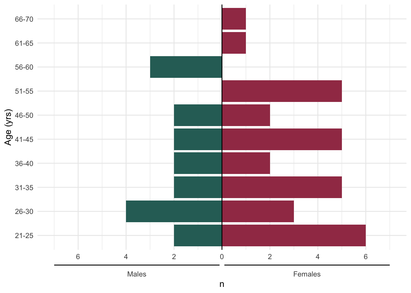
sex_lab <- primitive_bracket(
  key  = key_range_manual(          # <− positions + labels
    start = c(-7,0.1),
    end = c(-0.1,7),# -6  and  +6  on the x-axis
    name     = c("Males", "Females")
  ),
  position = "bottom"         # draw it at the bottom of the panel
)

Plot_demo <- 
data_devices_cleaned |>  
  mutate(
         age_group = 
           cut(age, 
               breaks = seq(15,70,5), 
               labels = c("18-20", "21-25", "26-30", "31-35", 
                          "36-40", "41-45", "46-50", "51-55", 
                          "56-60", "61-65", "66-70"),
               right = TRUE, ordered_result = TRUE),
         ) |> 
  group_by(sex, age_group) |> 
  dplyr::summarize(n = n(), .groups = "drop") |> 
  mutate(n = ifelse(sex == "Male", -n, n)) |> 
  ggplot(aes(x= age_group, y = n, fill = sex)) + 
  geom_col() +
  geom_hline(yintercept = 0) +
  scale_y_continuous(breaks = seq(-6,6, by = 2), 
                     labels = c(6, 4, 2, 0, 2, 4, 6)) +
  scale_fill_manual(values = c(Male = "#2D6D66", Female = "#A23B54")) + 
  guides(fill = "none", alpha = "none",
         x = guide_axis_stack(
           "axis", sex_lab
         )) +
  theme_minimal() +
  coord_flip(ylim = c(-7, 7)) +
  labs(x = "Age (yrs)", y = "n")

Plot_demo

ggsave("figures/Fig1_age.png", 
       width = 6, height = 6, units = "cm", scale = 1.6)

location_stats <- 
data_devices_cleaned |> 
  dplyr::summarise(
    tz = n_distinct(UTC_dev),
    country = n_distinct(country),
    n = n()
  ) |> 
  pivot_longer(
    cols = everything()
  ) |> 
  dplyr::mutate(name = case_match(name,
                           "country" ~ "Countries",
                           "tz" ~ "Time zones",
                           "n" ~ "Participants"),
         name = factor(name, levels = c("Time zones", "Countries", "Participants"))
         )

P_stats <-
location_stats |> 
  ggplot(aes(y = fct_rev(name), x = value, fill = name)) +
  geom_col() +
  geom_text(aes(label = value), color = "white", hjust = 1.2, fontface = 2, size = 3) +
  theme_minimal() +
  theme_sub_panel(grid = element_blank()) +
  theme_sub_axis_bottom(text = element_blank()) + 
  theme_sub_plot(background = element_rect(fill = alpha("white", 0.75))) +
  labs(x = NULL, y = NULL) +
  scale_fill_manual(values = c(`Time zones` = "deepskyblue3",
                               Participants = "red",
                               Countries = "grey")) +
  guides(fill = "none")

P_tz <-
  data_devices_cleaned |> 
    group_by(UTC_dev) |> 
    dplyr::summarise(n = n()) |> 
    ggplot(aes(x=UTC_dev, y = n)) +
    geom_vline(xintercept = 0, col = "grey") +
    geom_hline(yintercept = 0, col = "grey") +
    geom_col(fill = "deepskyblue3")+
    geom_text(aes(label = n), fontface = 2, vjust = -0.2) +
    theme_minimal() +
    theme_sub_panel(grid.major.y = element_blank(),
                    grid.minor = element_blank()) +
    theme_sub_axis_left(text = element_blank()) +
    scale_x_continuous(breaks = seq(-12, 12, 2)) +
    labs(x = "Deviation from UTC (h) on 22 Sep 2025", y = "n") +
    coord_cartesian(xlim = c(-11,11), ylim = c(NA, 30))

world <- ne_countries(scale = "medium", returnclass = "sf")
    
countries_colors <- tibble(
      country = data_devices_cleaned |> dplyr::count(country) |> pull(country),
      color   = "#0073C2FF",
      stringsAsFactors = FALSE
    )
    
world$color <- ifelse(
      world$name %in% countries_colors$country,
      countries_colors$country[match(world$name, countries_colors$country)],
      NA
    )
    
location_info <- tibble(
      country  = data_devices_cleaned |> pull(country),
      lat      = data_devices_cleaned |> pull(latitude),
      lon      = data_devices_cleaned |> pull(longitude),
      color    = "#0073C2FF",
      stringsAsFactors = FALSE
    ) |> 
  mutate(lat2 = plyr::round_any(lat, 12), 
         lon2 = plyr::round_any(lon, 12)) |> 
  dplyr::summarize(
    .by = c(lat2, lon2),
    lat = mean(lat),
    lon = mean(lon),
    color = unique(color),
    n = n()
  )
    
locations <- st_as_sf(location_info, coords = c("lon", "lat"), crs = 4326)
world_proj     <- st_transform(world,    crs = "+proj=eqc")
locations_proj <- st_transform(locations, crs = "+proj=eqc")
bb <- st_bbox(world_proj)
tz <- sf::st_read("data/tz_now/combined-shapefile-with-oceans-now.shp")  # or .gpkg / .geojson

Reading layer `combined-shapefile-with-oceans-now' from data source 
  `/Users/zauner/Documents/Arbeit/12-TUM/Repos_Misc/2025_ADayInDaylight/data/tz_now/combined-shapefile-with-oceans-now.shp' 
  using driver `ESRI Shapefile'
Simple feature collection with 92 features and 1 field
Geometry type: MULTIPOLYGON
Dimension:     XY
Bounding box:  xmin: -180 ymin: -90 xmax: 180 ymax: 90
Geodetic CRS:  WGS 84

tz_lines <- sf::st_boundary(tz)

P_map <-
  ggplot() +
  geom_sf(
    data = world_proj,
    # aes(fill = color),
    fill = "grey",
    color = NA,
    size = 0.25,
    alpha = 0.5,
    show.legend = FALSE
  ) +
  geom_sf(data = tz_lines,
          colour = "deepskyblue3",
          linewidth = 0.15) +
  geom_sf(
    data = locations_proj,
    aes(size = n),
    fill = "red",
    alpha = 0.9,
    shape = 21,
    color = "#0073C2FF",
    stroke = 0.2
  ) +
  geom_sf_text(
    data = locations_proj,
    aes(label = n),
    size = 1.5,
    fontface = 2,
    color = "white",
    alpha = 0.75
  ) +
  scale_fill_manual(values = rep("#0073C2FF", 15)) +
  scale_size_continuous(range = c(2, 5)) +
  theme_minimal() +
  theme(legend.position = "none") +
  labs(x = NULL, y = NULL) +
  coord_sf(expand = FALSE)

P_map_patch <- 
(P_map + inset_element(P_stats, 0.05, 0.05, 0.25, 0.25)) / P_tz + plot_layout(heights = c(4.4,1))

ggsave("figures/Fig2_location.pdf",P_map_patch,
       width = 15, height = 10, units = "cm", scale = 1.6)
ggsave("figures/Fig2_location.png",
       P_map_patch,
       width = 14, height = 9.5, units = "cm", scale = 1.6)

Import wearable data

Next, we import the light data. There are two devices in use: ActLumus and ActTrust we need to import them separately, as they are using different import functions. device_id with four number indicate the ActLumus devices, whereas with seven numbers the ActTrust. We add a column to the data indicating the Type of device in use. We also make sure that the spelling equals the supported_devices() list from LightLogR. Then we construct filename paths for all files.

c("ActLumus", "ActTrust") %in% supported_devices()

[1] TRUE TRUE

data_devices_cleaned <- 
data_devices_cleaned |> 
  dplyr::mutate(device_type = 
           case_when(
              str_length(device_id) == 4 ~ "ActLumus",
              str_length(device_id) == 7 ~ "ActTrust"
           ),
         file_path = glue("data/lightloggers/{device_id}.txt")
         )

data_devices_cleaned <- 
data_devices_cleaned |> 
  dplyr::mutate(
    data = purrr::pmap(list(x = device_type, y = file_path, z = tz_identifier), 
                       \(x, y, z) {
                         import_Dataset(device = x, filename = y, tz = z,
                                        silent = TRUE)
                       }
    )
  )

We end with one dataset per row entry. As the two ActTrust files do not contain a melanopic EDI column, we will use the photopic illuminance column LIGHT towards that end. As there are only two participants with this shortcoming, it will not influence results overduly.

data_devices_cleaned <- 
data_devices_cleaned |> 
  dplyr::mutate(
    data = purrr::map2(device_type, data, 
                       \(x,y) {
                         if(x == "ActTrust") {
                           y |> dplyr::rename(MEDI = LIGHT)
                         }
                         else y
                         }
                       )
  )

Further, the dataset in Malaysia had a device malfunction on 22 September and only worked from the 23 September onwards. As there are minimal differences between dates and very few datasets in that region, we will not dismiss that dataset but rather shift data by one day. We need to shift the data by another 8 hours backwards, as that dataset was stored in UTC time (for some reason).

data_devices_cleaned <- 
data_devices_cleaned |> 
  dplyr::mutate(
    data = purrr::map2(record_id, data, 
                       \(x,y) {
                         if(x == "25") {
                           y |> dplyr::mutate(
                             Datetime = Datetime - ddays(1) - dhours(8)
                             )
                         }
                         else y
                         }
                       )
  )

Light data

Cleaning light data

In this section we will prepare the light data through the following steps:

resampling data to 5 minute intervals
filling in missing data with explicit gaps
removing data that does not fall between 2025-09-21 10:00:00 UTC and 2025-09-23 12:00:00 UTC, which contains all times where 22 September occurs somewhere on the planet

data_devices <-
data_devices_cleaned |> 
  dplyr::mutate(
    data = purrr::map(data, 
                       \(x) {
                           x |> 
                           aggregate_Datetime("5 mins") |> #resample to 5 mins
                           gap_handler(full.days = TRUE) |> #put in explicit gaps
                           filter_Datetime(start = "2025-09-21 10:00:00",
                                           end = "2025-09-23 12:00:00",
                                           tz = "UTC") #cut out a section of data
                         }
                       )
  )

Next, we add a secondary Datetime column that runs on UTC time.

data_devices <-
data_devices |> 
  dplyr::mutate(
    data = purrr::map(data, 
                       \(x) {
                           x |> 
                           dplyr::mutate(Datetime_UTC = Datetime |> force_tz("UTC"))
                         }
                       )
  )

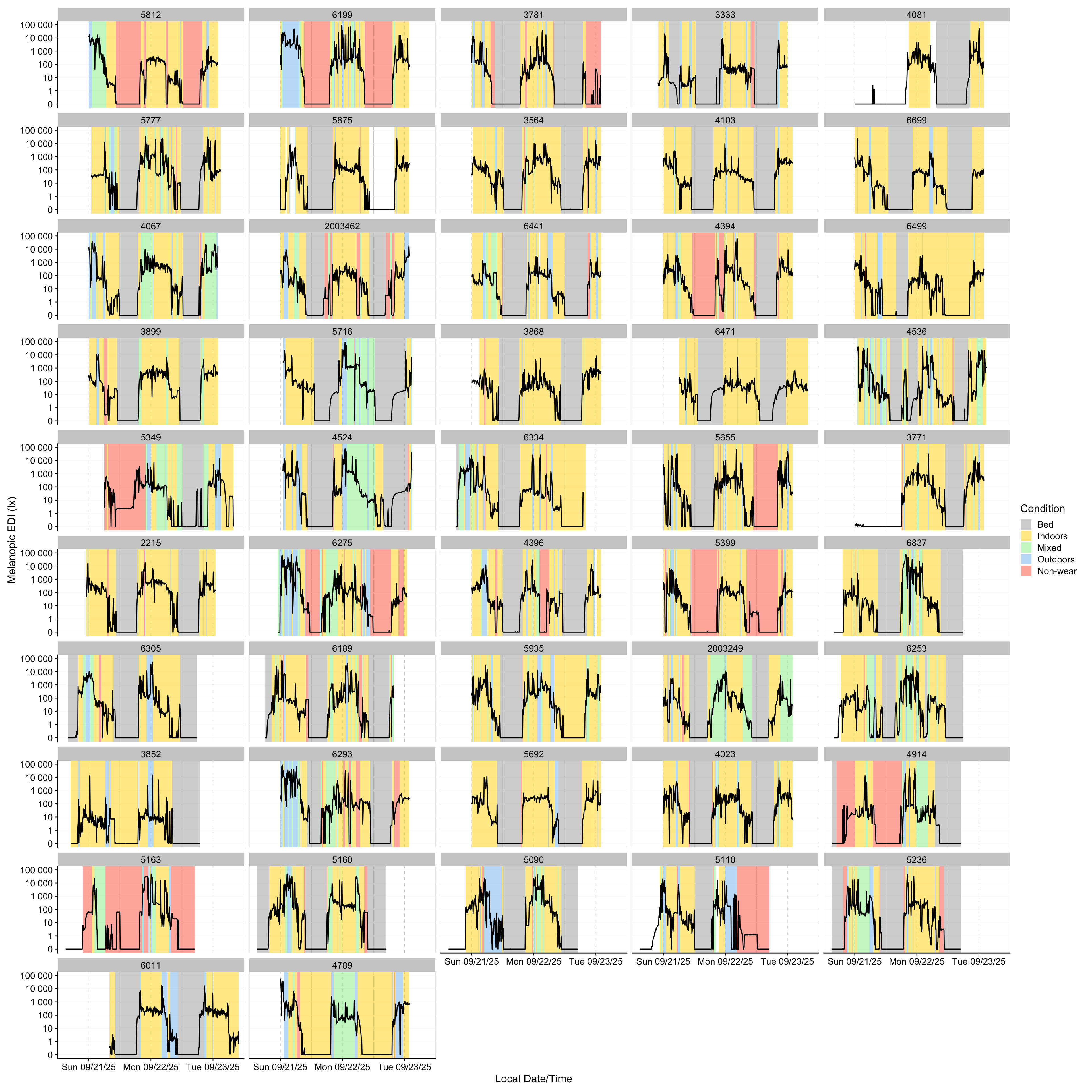
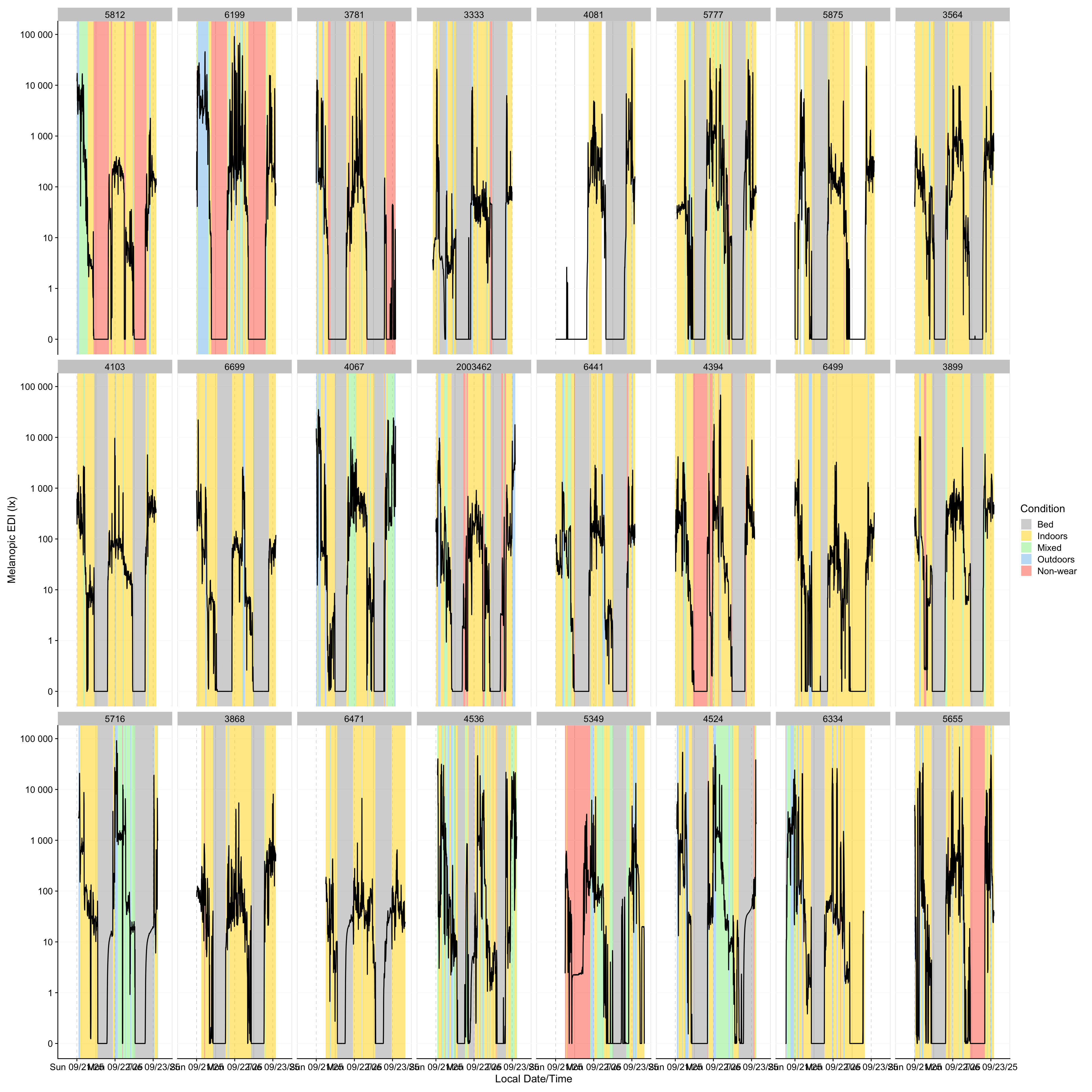
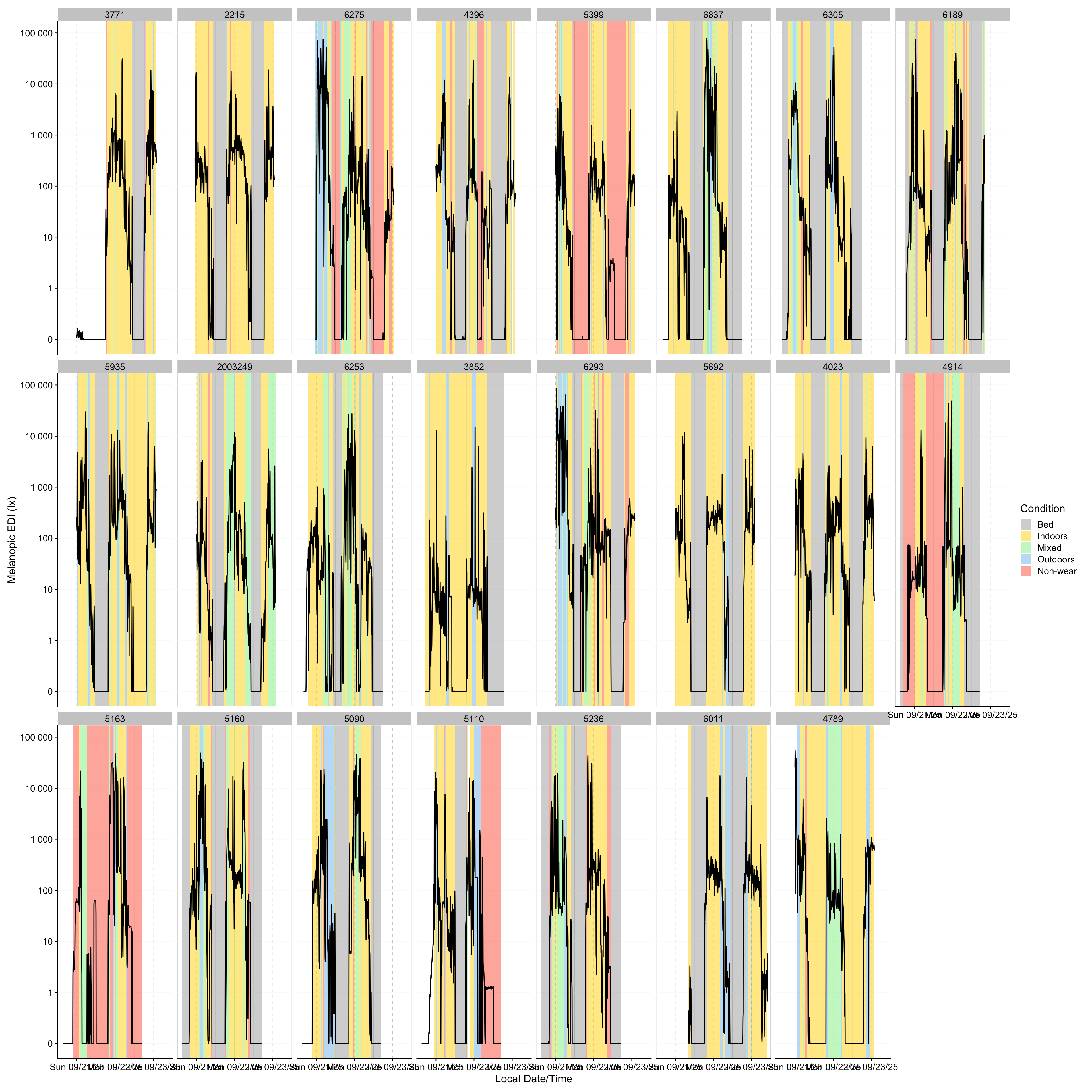
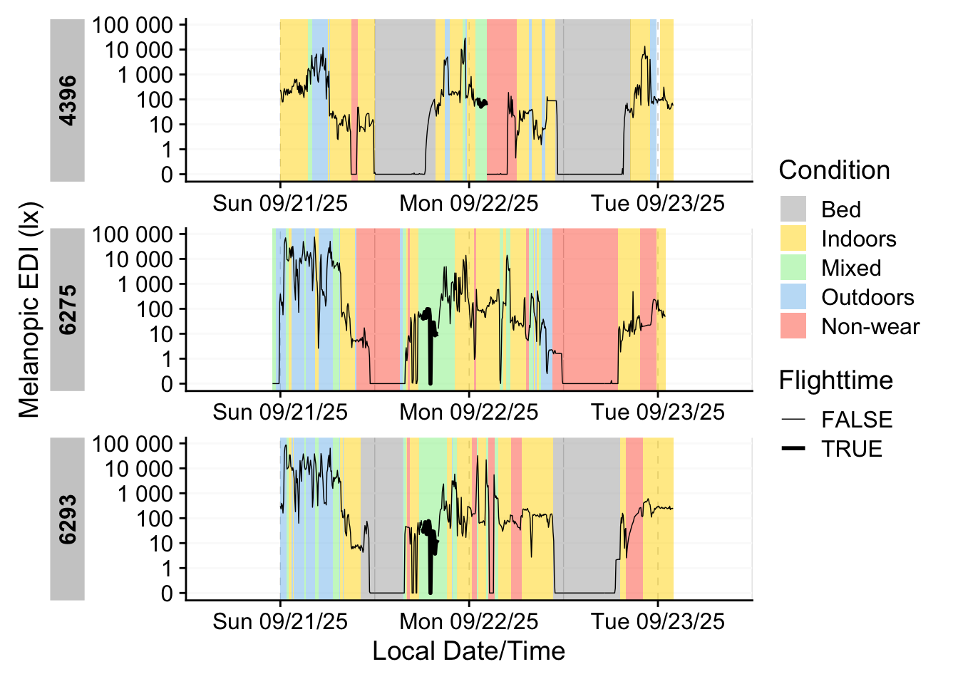
Visualizing light data

Now we can visualize the whole dataset - first by combining all datasets.

start_dt <- as.POSIXct("2025-09-21 10:00:00", tz = "UTC")
start_dt2 <- as.POSIXct("2025-09-22 00:00:00", tz = "UTC")
end_dt <- as.POSIXct("2025-09-23 12:00:00", tz = "UTC")
end_dt2 <- as.POSIXct("2025-09-23 00:00:00", tz = "UTC")

light_data <- 
  join_datasets(!!!data_devices$data) |> 
  mutate(Datetime = Datetime |> with_tz("UTC"))

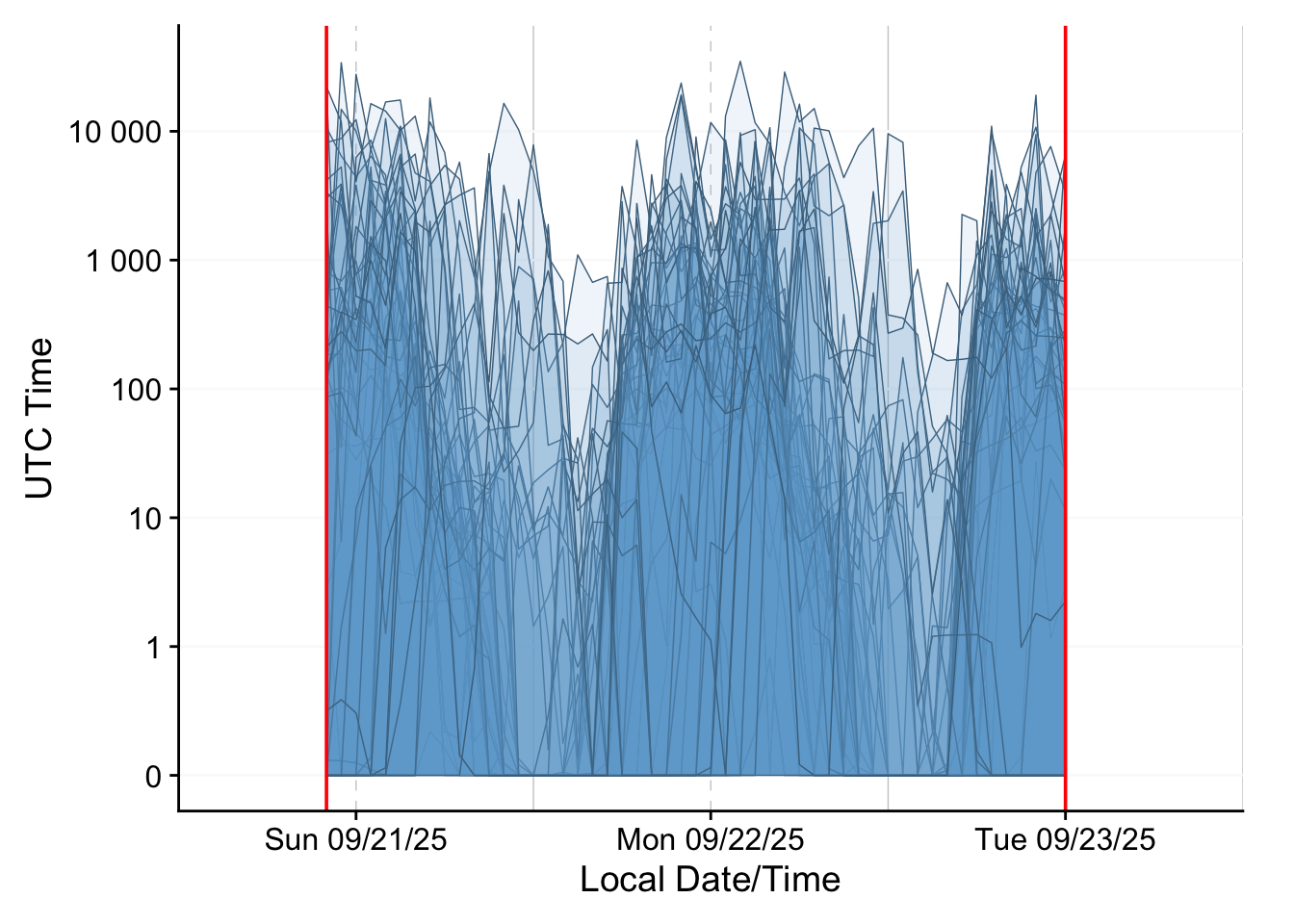
light_data |> 
  aggregate_Datetime("1hour") |> 
  gg_days(facetting = FALSE, 
          group = Id, 
          geom = "ribbon",
          lwd = 0.25,
          fill = "skyblue3",
          color = "skyblue4",
          alpha = 0.1,
          y.axis.label = "UTC Time"
          ) +
  geom_vline(xintercept = c(start_dt, end_dt), color = "red")

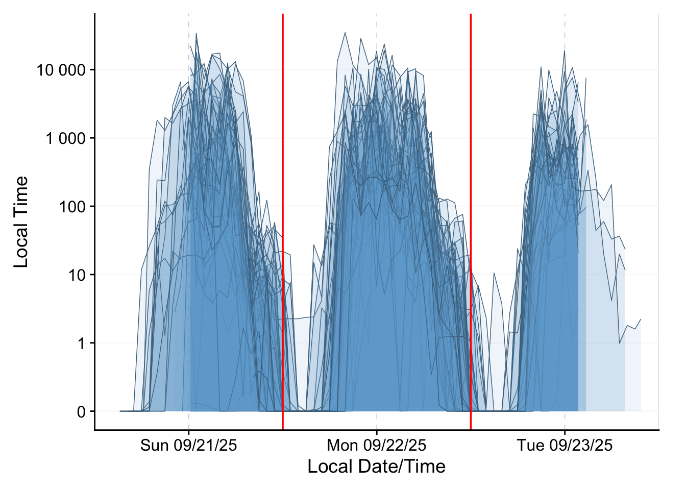
light_data |> 
  aggregate_Datetime("1hour") |> 
  gg_days(Datetime_UTC,
          geom = "ribbon",
          facetting = FALSE,
          fill = "skyblue3",
          color = "skyblue4",
          alpha = 0.1,
          group = Id, 
          lwd = 0.25,
          y.axis.label = "Local Time"
          ) +
  geom_vline(xintercept = c(start_dt2, end_dt2), color = "red")

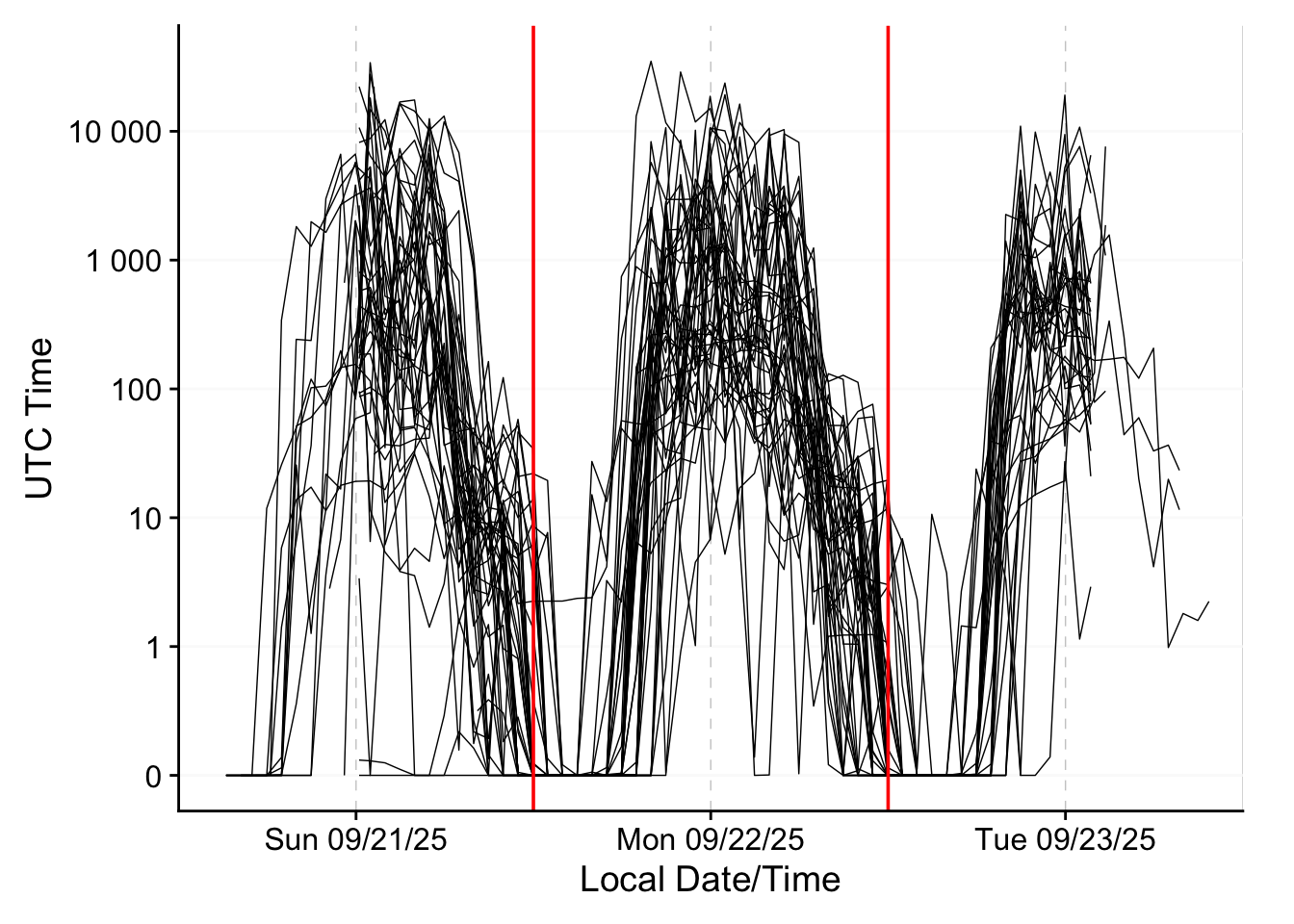
light_data |> 
  aggregate_Datetime("1hour") |> 
  gg_days(Datetime_UTC,
          facetting = FALSE, 
          group = Id, 
          lwd = 0.25,
          y.axis.label = "UTC Time"
          ) +
  geom_vline(xintercept = c(start_dt2, end_dt2), color = "red")

boundaries <- tibble(
  start = c(start_dt, start_dt2),
  end = c(end_dt, end_dt2),
  name = c("UTC Time", "Local Time")
)

p <- 
light_data |> 
  aggregate_Datetime("2 hours") |>
  select(Id, Datetime, Datetime_UTC, MEDI) |> 
  pivot_longer(-c(Id, MEDI)) |> 
  mutate(name = case_match(name,
                           "Datetime" ~ "UTC Time",
                           "Datetime_UTC" ~ "Local Time")) |> 
  dplyr::mutate(name = factor(name)) |> 
    gg_days(value,
            geom = "ribbon",
            fill = "skyblue3",
            alpha = 0.4,
            color = "black",
          facetting = FALSE, 
          group = Id, 
          lwd = 0.1,
          x.axis.label = "{next_state} {if(transitioning) '(transitioning)' else ''}",
          y.axis.label = "Melanopic EDI (lx)",
          x.axis.breaks = \(x) Datetime_breaks(x, by = "6 hours", shift = 0),
          x.axis.format = "%H:%M"
    )  + 
  geom_vline(data = boundaries, aes(xintercept=start), col = "red", lty = 2, inherit.aes = FALSE)+
  geom_vline(data = boundaries, aes(xintercept=end), col = "red", lty = 2, inherit.aes = FALSE)+
  geom_segment(data = boundaries, 
               aes(y = 25000, x = start, xend = end), 
               arrow = arrow(length = unit(0.1, "inches"), ends = "both"), col = "red",  
               inherit.aes = FALSE)+
  annotate(geom = "text", y = 25000, x = mean(c(start_dt2, end_dt2)), 
           vjust = -0.4, label = "Global 22 September", col = "red") +
  transition_states(
    name, 
    transition_length = 1,
    state_length = 1
  )

if(interactive()){
animation <- 
animate(p, width = 1200, height = 700, res = 150)

animation

anim_save("figures/patterns.gif", animation)
}

Events

Cleaning events

In this section we deal with with the activity logs - first by filtering them out of the dataset, and selecting the relevant aspects.

events <- 
data |> 
  filter(redcap_repeat_instrument == "log_a_new_activity") |> 
  select(record_id,
         type.factor, 
         social_context.factor,
         wear_activity.factor,
         nonwear_activity.factor,
         nighttime.factor,
         setting_level01.factor, 
         setting_level02_indoors.factor,
         setting_level02_indoors_home.factor,
         setting_level02_indoors_workingspace.factor,
         setting_level02_indoors_healthfacility.factor,
         setting_level02_indoors_learningfacility.factor,
         setting_level02_indoors_leisurespace.factor,
         setting_level02_indoors_retailfacility.factor,
         setting_level02_mixed.factor,
         setting_level02_outdoors.factor,
         lighting_scenario_daylight___1.factor,
         lighting_scenario_daylight___2.factor,
         lighting_scenario_daylight___3.factor,
         lighting_scenario_daylight___4.factor,
         lighting_scenario_3___1.factor,
         lighting_scenario_3___2.factor,
         lighting_scenario_3___3.factor,
         lighting_scenario_2___1.factor,
         lighting_scenario_2___2.factor,
         lighting_scenario_2___3.factor,
         lighting_scenario_2___4.factor,
         autonomy.factor,
         notes, 
         startdate, enddate
         )

#adding labels to the factors
label(events$type.factor) = "Wear type: Are you wearing the light logger at the moment?"
label(events$social_context.factor) = "Are you alone or with others?"
label(events$wear_activity.factor) = "Wear activity "
label(events$nonwear_activity.factor) = "Non-wear activity"
label(events$nighttime.factor) = "Where was the light logger when you were asleep?"
label(events$setting_level01.factor) = "Select the setting"
label(events$setting_level02_indoors.factor) = "Indoors setting"
label(events$setting_level02_indoors_home.factor) = "Indoors setting (home)"
label(events$setting_level02_indoors_workingspace.factor) = "Indoors setting (working space)"
label(events$setting_level02_indoors_learningfacility.factor) = "Indoors setting (learning facility)"
label(events$setting_level02_indoors_retailfacility.factor) = "Indoors setting (retail facility)"
label(events$setting_level02_indoors_healthfacility.factor) = "Indoors setting (health facility)"
label(events$setting_level02_indoors_leisurespace.factor) = "Indoors setting (leisure space)"
label(events$setting_level02_outdoors.factor) = "Outdoors setting"
label(events$setting_level02_mixed.factor) = "Indoors-outdoors setting"
label(events$lighting_scenario_daylight___1.factor) = "Select lighting setting (daylight) (choice=Outdoors (direct sunlight))"
label(events$lighting_scenario_daylight___2.factor) = "Select lighting setting (daylight) (choice=Outdoors (in shade / cloudy))"
label(events$lighting_scenario_daylight___3.factor) = "Select lighting setting (daylight) (choice=Indoors (near window / exposed to daylight))"
label(events$lighting_scenario_daylight___4.factor) = "Select lighting setting (daylight) (choice=Indoors (away from window))"
label(events$lighting_scenario_3___1.factor) = "Select lighting setting (electric light) (choice=Lights are switched on)"
label(events$lighting_scenario_3___2.factor) = "Select lighting setting (electric light) (choice=Low-light or dimmed lights)"
label(events$lighting_scenario_3___3.factor) = "Select lighting setting (electric light) (choice=Completed darkness)"
label(events$lighting_scenario_2___1.factor) = "Select lighting setting (screen use) (choice=Smartphone)"
label(events$lighting_scenario_2___2.factor) = "Select lighting setting (screen use) (choice=Tablet)"
label(events$lighting_scenario_2___3.factor) = "Select lighting setting (screen use) (choice=Computer)"
label(events$lighting_scenario_2___4.factor) = "Select lighting setting (screen use) (choice=Television)"
label(events$autonomy.factor) = "Were the lighting conditions in this setting self-selected (i.e., you had control over lighting intensity, spectrum, or exposure)?"

Next, we condense columns that can be expressed as one. We also lose the .factor extension, as now all doubles are removed. Finally, we simplify entries.

events <- 
events |> 
  rename_with(\(x) x |> str_remove(".factor")) |> #remove .factor extension
  dplyr::mutate(
    type = type |> fct_relabel(\(x) str_remove(x, "-time| time| \\(not wearing light logger\\)")),
    across(c(wear_activity, setting_level01),
           \(x) x |> fct_relabel(\(y) str_remove(y, " \\(.*\\)"))
           ),
    nonwear_activity = 
      nonwear_activity |> fct_recode(
        "Dark mobile" = "Left in a bag, or other mobile dark place",
        "Dark stationary" = "Left in a drawer or cabinet, or other stationary dark place",
        "Stationary" = "Left on a table or other surface with varying light exposure"
      ),
    nighttime = 
      nighttime |> fct_recode(
        "Upward" = "Facing upward on bedside table",
        "Downward" = "Facing downward on bedside table"
      ),
    across(c(setting_level02_indoors, setting_level02_outdoors),
           \(x) x |> fct_recode(
        "Leisure" = "Leisure space (sports, recreation, entertainment)",
        "Commercial" = "Retail, food or services facility",
        "Workplace" = "Working space",
        "Education" = "Learning facility",
        "Healthcare" = "Health facility"
           )
        ),
    setting_level01 = 
      setting_level01 |> fct_recode(
        "Mixed" = "Indoor-outdoor setting"
      ),
    autonomy =
      autonomy |> fct_recode(
        Yes = "Yes, fully self-selected (e.g., adjusting lights at home or in a private office, moving to shaded area)",
        Partly = "Partly self-selected (e.g., some control such as opening blinds or switching a desk lamp, but not over main lighting)",
        No = "Not self-selected (e.g., public transport, shared office, classroom, hospital, airplane, etc.)",
        NULL = "Not applicable"
      )
  ) |> 
  dplyr::rename(setting_light = setting_level01)

events <- 
events |>
  dplyr::mutate(
    scenario_daylight =
      case_when(
        (lighting_scenario_daylight___1 == "Checked") & 
          (setting_light %in% c("Outdoors", "Mixed")) ~ "Direct sunlight",
        (lighting_scenario_daylight___2 == "Checked") &
          (setting_light %in% c("Outdoors", "Mixed")) ~ "Shade / cloudy",
        (lighting_scenario_daylight___3 == "Checked") &
          (setting_light %in% c("Indoors", "Mixed")) ~ "Near a window",
        (lighting_scenario_daylight___4 == "Checked") &
          (setting_light %in% c("Indoors", "Mixed")) ~ "Away from window"
      ),
    scenario_electric =
      case_when(
        lighting_scenario_3___3 == "Checked" ~ "Lights off",
        lighting_scenario_3___2 == "Checked" ~ "Dim light",
        lighting_scenario_3___1 == "Checked" ~ "Lights on",
      ),
    across(starts_with("lighting_scenario_2___"),
           \(x) ifelse(x == "Checked", TRUE, FALSE)),
  ) |> 
  dplyr::rename(screen_phone = lighting_scenario_2___1,
                screen_tablet = lighting_scenario_2___2,
                screen_pc = lighting_scenario_2___3,
                screen_tv = lighting_scenario_2___4
                ) |> 
  select(-starts_with("lighting_scenario")) |> 
  dplyr::mutate(
    wear_activity = case_when(type == "Wear" ~ wear_activity, .default = NA),
    nonwear_activity = case_when(type == "Non-wear" ~ nonwear_activity, .default = NA),
    nighttime = case_when(type == "Bedtime" ~ nighttime, .default = NA),
    setting_level02_mixed = case_when(setting_light == "Mixed" ~ setting_level02_mixed, .default = NA),
    setting_level02_indoors = case_when(setting_light == "Indoors" ~ setting_level02_indoors, .default = NA),
    setting_level02_outdoors = case_when(setting_light == "Outdoors" ~ setting_level02_outdoors, .default = NA),
    setting_level02_indoors_leisurespace = case_when(setting_level02_indoors == "Leisure" ~ setting_level02_indoors_leisurespace, .default = NA),
    setting_level02_indoors_workingspace = case_when(setting_level02_indoors == "Workplace" ~ setting_level02_indoors_workingspace, .default = NA),
  ) |> 
  unite("type.detail", c(wear_activity, nonwear_activity, nighttime), na.rm = TRUE,
        remove = FALSE) |> 
  unite("setting_location", 
        c(setting_level02_indoors, setting_level02_outdoors, setting_level02_mixed), 
        na.rm = TRUE, remove = FALSE) |> 
  unite("setting_specific", 
        starts_with("setting_level02_indoors_"), 
        na.rm = TRUE, remove = FALSE) |> 
  dplyr::rename_with(\(x) x |> str_remove("_level02")) |> 
  relocate(scenario_daylight, scenario_electric, .before = screen_phone) |> 
  relocate(startdate, .before = 1) |> 
  select(-enddate) |> 
  dplyr::mutate(
    across(c(setting_location, setting_specific, type.detail),
           \(x) fct_recode(x, NULL = ""))
  )

part_data <- data_devices |> select(-data) |> mutate(record_id = as.character(record_id))

events_complete <- 
events |> 
  dplyr::mutate(record_id = as.character(record_id)) |> 
  left_join(part_data, by = "record_id") |> 
  drop_na(tz_identifier)

label(events_complete$record_id) = "Record ID"

events_complete <- 
events_complete |> 
  dplyr::mutate(
    Datetime = as.POSIXct(startdate, tz = "UTC"),
    UTC_dt = force_tzs(Datetime, tz_identifier),
    .before = 1) |> 
  select(-startdate)

Summaries

In this section we will calculate some summary statistics regarding events

events_complete <- 
events_complete |> 
  dplyr::mutate(status.duration = c(diff(Datetime), na_dbl), 
                .by = record_id,
                .after = Datetime) |> 
  filter(!record_id %in% c("31", "30", "44"))

label(events_complete$status.duration) = "Time between log entries"
label(events_complete$type.detail) = "Wear/Non-wear context"
label(events_complete$setting_location) = "General setting"
label(events_complete$setting_specific) = "Specific indoor setting"
label(events_complete$scenario_daylight) = "Daylight conditions"
label(events_complete$scenario_electric) = "Electric lighting conditions"
label(events_complete$screen_phone) = "Phone use"
label(events_complete$screen_tablet) = "Tablet use"
label(events_complete$screen_pc) = "Computer use"
label(events_complete$screen_tv) = "Television use"
label(events_complete$sex) = "Sex"
label(events_complete$city) = "City"
label(events_complete$country) = "Country"
label(events_complete$latitude) = "Latitude"
label(events_complete$longitude) = "Longitude"
label(events_complete$tz_identifier) = "Time zone identifier"
label(events_complete$UTC_dev) = "Time zone deviation from UTC"
label(events_complete$device_type) = "Used device"
label(events_complete$file_path) = "File path"
label(events_complete$setting_indoors) = "Indoor settings"
label(events_complete$setting_outdoors) = "Outdoor settings"
label(events_complete$setting_mixed) = "Outdoor-Indoor mixed settings"
label(events_complete$wear_activity) = "Activity"
label(events_complete$nonwear_activity) = "Non-wear wearable position"
label(events_complete$nighttime) = "Nightstand wearable measurement direction"

event_summary1 <- 
events_complete |> 
  dplyr::summarize(.by = record_id,
            n = n(),
            mean.duration = mean(status.duration, na.rm = TRUE),
            covered.timespan = last(Datetime) - first(Datetime)
  )
label(event_summary1$n) = "Log entries"
label(event_summary1$mean.duration) = "Mean duration between log entries"
units(event_summary1$mean.duration) = "hours"
label(event_summary1$covered.timespan) = "Total time span of log entries"

event_summary1.tbl <- 
event_summary1 |> 
  tbl_summary(include = -record_id,
              statistic = list(all_continuous() ~ "{mean} ({min}-{max})")
              ) |> 
  modify_caption("**Activity logging (by-participant level)**")

event_summary1.tbl

**Activity logging (by-participant level)**
Characteristic	N = 47¹
Log entries	38 (9-80)
Mean duration between log entries	1.69 hours (0.53 hours-3.92 hours)
Total time span of log entries	2.09 days (1.14 days-4.13 days)
¹ Mean (Min-Max)

gtsave(event_summary1.tbl |> as_gt(), "tables/table1.png")

file:////var/folders/9p/326_k3kx43qbn_cyl1rqfhb00000gn/T//RtmpQk3ZUL/file5ad9452f1ac4.html screenshot completed

event_tbl_setting <- 
events_complete |> 
  select(setting_indoors, setting_outdoors, setting_mixed
         ) |> 
  tbl_summary(missing = "no"
  )

event_tbl_setting

Characteristic	N = 1,763¹
Indoor settings
Home	661 (70%)
Workplace	126 (13%)
Education	17 (1.8%)
Commercial	84 (8.9%)
Healthcare	3 (0.3%)
Leisure	23 (2.4%)
Other	27 (2.9%)
Outdoor settings
Home	51 (15%)
Workplace	24 (6.8%)
Education	8 (2.3%)
Commercial	19 (5.4%)
Healthcare	0 (0%)
Leisure	83 (24%)
Other	166 (47%)
Outdoor-Indoor mixed settings
Covered patio or terrace	20 (8.1%)
Semi-open corridor/gallery	11 (4.5%)
Balcony	3 (1.2%)
Veranda	5 (2.0%)
Atrium	1 (0.4%)
Transportation (car/taxi)	138 (56%)
Transportation (bus or commuter/regional rail)	31 (13%)
Transportation (long-distance train)	6 (2.4%)
Transportation (underground, subway)	6 (2.4%)
Transportation (airplane)	6 (2.4%)
Transportation (bike)	5 (2.0%)
Transportation (ferry)	1 (0.4%)
Other	14 (5.7%)
¹ n (%)

gtsave(event_tbl_setting |> as_gt(), "tables/table2.png")

file:////var/folders/9p/326_k3kx43qbn_cyl1rqfhb00000gn/T//RtmpQk3ZUL/file5ad944f8e420.html screenshot completed

event_tbl_indoors <- 
events_complete |> 
  select(setting_specific
         ) |> 
  tbl_summary(missing = "no"
  )

event_tbl_indoors

Characteristic	N = 1,763¹
Specific indoor setting
Bathroom	86 (9.6%)
Bedroom	114 (13%)
Break/lounge area	6 (0.7%)
Classroom	4 (0.4%)
Conference/meeting room	18 (2.0%)
Convenience store/supermarkt	23 (2.6%)
Corridor	10 (1.1%)
Dentist	1 (0.1%)
Drug store	1 (0.1%)
Home office	85 (9.5%)
Kitchen	100 (11%)
Laboratory	2 (0.2%)
Lecture hall	2 (0.2%)
Library	2 (0.2%)
Living room	213 (24%)
Office supply store	1 (0.1%)
Open-plan office area	16 (1.8%)
Other	80 (8.9%)
Parking garage	10 (1.1%)
Personal workspace/desk	72 (8.0%)
Restaurant/cafeteria/bakery	32 (3.6%)
Shopping mall	16 (1.8%)
Studio	1 (0.1%)
¹ n (%)

gtsave(event_tbl_indoors |> as_gt(), "tables/table3.png")

file:////var/folders/9p/326_k3kx43qbn_cyl1rqfhb00000gn/T//RtmpQk3ZUL/file5ad930491440.html screenshot completed

event_tbl_wear <- 
events_complete |> 
  select(type, wear_activity, nonwear_activity, nighttime
         ) |> 
  tbl_summary(
    missing = "no"
  )

event_tbl_wear

Characteristic	N = 1,763¹
Wear type: Are you wearing the light logger at the moment?
Wear	1,535 (87%)
Non-wear	132 (7.5%)
Bedtime	88 (5.0%)
Activity
Sedentary	728 (47%)
Light activity	693 (45%)
Moderate activity	103 (6.7%)
High-intensity activity	11 (0.7%)
Non-wear wearable position
Dark stationary	13 (9.8%)
Dark mobile	22 (17%)
Stationary	88 (67%)
Other	9 (6.8%)
Nightstand wearable measurement direction
Upward	78 (89%)
Downward	5 (5.7%)
Other	5 (5.7%)
¹ n (%)

gtsave(event_tbl_wear |> as_gt(), "tables/table4.png")

file:////var/folders/9p/326_k3kx43qbn_cyl1rqfhb00000gn/T//RtmpQk3ZUL/file5ad9dd08e84.html screenshot completed

event_tbl_other <- 
events_complete |> 
  select(social_context, setting_light, scenario_daylight, 
         scenario_electric, autonomy
         ) |> 
  tbl_summary(
    missing_text = "Missing"
  )

event_tbl_other

Characteristic	N = 1,763¹
Are you alone or with others?
Alone	1,028 (59%)
With others	728 (41%)
Missing	7
Select the setting
Indoors	941 (61%)
Outdoors	351 (23%)
Mixed	247 (16%)
Missing	224
Daylight conditions
Away from window	363 (25%)
Direct sunlight	216 (15%)
Near a window	664 (46%)
Shade / cloudy	210 (14%)
Missing	310
Electric lighting conditions
Dim light	242 (19%)
Lights off	356 (28%)
Lights on	658 (52%)
Missing	507
autonomy
Yes	825 (58%)
Partly	172 (12%)
No	428 (30%)
Missing	338
¹ n (%)

gtsave(event_tbl_other |> as_gt(), "tables/table4.png")

file:////var/folders/9p/326_k3kx43qbn_cyl1rqfhb00000gn/T//RtmpQk3ZUL/file5ad9773c8331.html screenshot completed

label(data$situation_logging_difficulty) = "Situations where logging was difficult  Were there specific times, activities, or situations when you could not log or found it hard to log?"

table_difficulties <- 
data |> 
  filter(!is.na(situation_logging_difficulty) & situation_logging_difficulty != "") |> 
  filter(!is.na(device_id)) |> 
  select(device_id, situation_logging_difficulty) |> 
  gt() |> 
  tab_style(locations = cells_column_labels(), style = cell_text(weight = "bold")) |> cols_align("left")

table_difficulties

Device ID	Situations where logging was difficult Were there specific times, activities, or situations when you could not log or found it hard to log?
5812	Sunday afternoon: attended horseriding competition and travelling back and cleaning up afterwards. Otherwise: sometimes difficult to log for very short activities (e.g. picking something up from the basement), where logging would take as long as logging, this made me not log the activity
6199	When I was moving at the university from one building to another only for a minutes.
3781	I found it difficult to track every movement within my apartment. Therefore I didn't track all of those 'micro-movements' (e.g. bedroom - bath - kitchen - livingroom - kitchen...). I also forgot to log in for my 'after-lunch' walk (was on the phone when leaving).
3333	I did not encounter any challenges in logging.
4081	In principle, it was difficult for me to find the correct options. Overall, it was regular office work with just one break.
5777	movement at home between rooms, quick location change
5875	Yes, for instance in the morning rush at home where my location within the house changed rapidly (going back and forth between rooms). I also often remembered too late when biking to work and arriving at work, that I needed to log. I did, but often too late as I was busy getting my bike, putting it away, etc.
3564	In general it was a pity that one could not log events afterwards. Thus, I often forgot to log an event and could not fix this error.
4103	The logging took quite some time. So times where quick logging was neccessary it became difficult, e.g. in train stations or similar.
6699	while on the phone with someone and exiting/entering different locations e.g. from outdoors into supermarket and back out.
4067	The way between apartement and car. The ways between office at work.
2003462	During travel using public transport
6441	Transitional states were hard to log, often because I would either forget about it, or do it during the actual transitional state which meant it was over by the time I'd finished logging. Logging during stressful or busy moments (i.e. catching a train, etc.) which require a lot of bandwidth was also hard.
4394	The activity log is well designed in case the activity / the location do not change too often. However, for activities/locations that change frequently, the activity log is time-consuming. It is difficult to believe that subjects in a field study would comply.
6499	I fell asleep unintentionally - leaving the device on until I woke up in the middle of the night. I did not log nighttime awakenings because taking the phone out would've been interfering with falling back asleep.
3899	way to the car (less than 1 minute)
5716	When I was constantly getting in the car or out of the car, I was nervous that I would forget some of the logging. (I was looking for a house, so I was constantly going to new places.)
3868	I did not log while changing rooms inside my flat
6471	1. Since I live in a studio-style room, it's difficult to separate areas such as home office, bedroom, and living room. 2. How should I define the distance from the window in order to count as 'away from window'? 3. I sometimes felt confused when logging the indoor-outdoor setting.
4536	Yeah there were some activities that i could not find exact correspondance throughout the options.
5349	Logging itself was not difficult, but there were times I only remembered to log after transitioning or when in the midst of the transition, rathet than at the point of transition.
4524	some options were not comprehensive enough (eg. motorcycle couldn't be count as a vehicle but riding a motorcycle also not a physical activity such as walking)
6334	Yes - on the evening of 9/22 (the last night) I was unable to log the time I took off the Actlumus and put it on my bedside table for sleep because the my cap survey would not load after multiple attempts. For reference, I put my Actlumus device facing up at 22:30 on 9/22. Otherwise I was able to log activities.
5655	Taking care of newborn and moving to another light environment a few times were challenging for logging due to the urgency of diaper change/crying/other things.
3771	shorttime changing of scenes (transitions between buildings), shorter activities
3887	Short transition times like walking to my car or from the car to the gym.
2215	I found it challenging to accurately log light exposure when moving between rooms (at home) - especially because the illumination always seems to be very uniform in my home. I also believe my self-reported screen time, especially smartphone use, was likely underestimated.
6275	Yes, I was on a trip so when we went down the bus and up again and when the change of activity was short, for example during housework activities.
4396	When quickly changing environment. E.g. going in to a small grocery store for 2 minutes and then go out again. There were a bit too many questions.
5399	When it was raining a lot, and cold to be holding the phone outside.
6837	Not really.
6305	Yes, my phone got locked and I couldn't log my activity between 3 p.m. and 11 p.m. However, it was a problem with my phone and not with the application.
6189	When running errands in the car. I would drive somewhere, pop into a store, and get back on the car. I think there was at least one time I realized I had not logged in going into the store when I was already getting back into the car. Also, I when moving around the house doing chores. I had not notice before how different is the amount of natural light across my house.
5935	engaging in multiple activities within a short time window were challenging to register. Moreover, I had to teach and had multiple meetings on Monday. I wasn't able to register all small activities like quicly grab a tea while working
2003249	No
6253	I tried to log all my activities, but sometimes I was changing my space a lot, for instance when I was getting ready to go out.
5308	I was with people I do not see in person very often. It was not hard to log and they were interested in the project but there were a few moments when we changed locations while talking and walking and I forgot to add to the log. I retrospectively noted these situations in the comments (e.g., left 10 minutes ago)
3852	no, available to log for all behaviors/change in environment.
6293	when the change of activity was for less than 2-3 min. For instance, from the car- park at home or at work walking to the house or the office (it takes 20-30 seconds max)
5692	There were some uncertainties and I kind of adapted.
4023	I forgot two or three times to log, when catching the train / walking just a very short time outside and been in conversation or in thoughts. I did not track my movements at home, because I was walking around quite much with kid, cooking, cleaning and so on.
4914	There were times when I transitioned quickly, such as getting in a car to drive to one location briefly, and then to another, or times when I got in my car to drive home, and then was too busy to log each transition point.
5163	Yes, the first day (Sunday PDT) I was moving between accommodations, so I had to carry a lot of stuff back and forth outside and inside and into the car and then also bike while carrying other things... It was very hectic and almost impossible to properly log...
5160	I was doing a lot of chores around the house (I recently moved) so I was going from room to room constantly. I didn't update the location upon each change, but I'm sure there were light changes, though very quick. I also would drive and have quick walks outside to get to my car - I didn't log these separately, but hopefully it is not too unclear. Also, I was using my phone to log responses, but didn't typically include light from phone as something as I was only using it to log my entry. I hope that was the right choice! I changed locations (like drove somewhere new) and didn't log exactly where I ended up, but trying to give that information here now.
5090	Moving around the house - impossible to log going into different rooms while doing 'light chores'. Street shopping - I had to keep stopping every time I went into/out of a shop (book store, bakery, etc.) for only a few minutes at a time, and with only a few minutes on the sidewalk outside between each shop.
5110	At my workplace, there was no cellular service. As a result, I had to log my tasks at work retrospectively. I also forgot to put my actlumus back on 9/22 (~3:00 PST) due it constantly falling off.
5236	It wasn't difficult, it was inconvenient.
6011	Very brief changes in state (eg going into the lab briefly from my office), or transitions that happened back to back, eg, sometimes when I would arrive at work I would get chatting to a colleague and not log the arrival immediately (after having logged leaving home fine).
4789	Cleaning the apartment (fast changes of rooms and lighting conditions)

gtsave(table_difficulties, "tables/table_difficulties.png")

file:////var/folders/9p/326_k3kx43qbn_cyl1rqfhb00000gn/T//RtmpQk3ZUL/file5ad93c8f9c75.html screenshot completed

event_tbl_duration <-
events_complete |> 
  # drop_na(setting_light) |>
  dplyr::mutate(setting_light = 
                  case_when(type == "Bedtime" ~ "Bed",
                            type == "Non-wear" ~ "Non-wear",
                            .default = setting_light |> as.character()),
                setting_light = 
                  setting_light |> factor(levels = c("Bed", "Indoors", "Mixed", "Outdoors", "Non-wear"))) |> 
  dplyr::summarize(`Daily duration` = sum(status.duration, na.rm = TRUE),
                   .by = c(setting_light, record_id)) |> 
  dplyr::summarize(`Daily duration` = mean(`Daily duration`),
                   .by = c(setting_light)) |> 
  dplyr::mutate(`Daily duration` =
                  `Daily duration` /
                  sum(as.numeric(`Daily duration`)) *
                  24*60*60,
                Percent = 
                  (as.numeric(`Daily duration`)/
                  sum(as.numeric(`Daily duration`)))
                  # vec_fmt_percent()
                ) |> 
  arrange(setting_light) |> 
  gt(rowname_col = "setting_light") |> 
  grand_summary_rows( 
                     fns = list(
      sum ~ sum(.)
    ),
    fmt = list(~ fmt_percent(., columns = Percent, decimals = 0), 
               ~ fmt_duration(., columns = `Daily duration`, 
               input_units = "secs",
               max_output_units = 2))
    ) |> 
  fmt_duration(`Daily duration`, 
               input_units = "secs",
               max_output_units = 2) |> 
  fmt_percent(columns = Percent, decimals = 0) |> 
  sub_missing() |> 
  tab_header(title = "Mean daily duration in condition")

event_tbl_duration

Mean daily duration in condition
	Daily duration	Percent
Bed	5h 59m	25%
Indoors	10h 6m	42%
Mixed	1h 56m	8%
Outdoors	1h 31m	6%
Non-wear	2h 59m	12%
—	1h 25m	6%
sum	1d	100%

gtsave(event_tbl_duration, "tables/table5.png")

file:////var/folders/9p/326_k3kx43qbn_cyl1rqfhb00000gn/T//RtmpQk3ZUL/file5ad9383fd79e.html screenshot completed

Combining Events with light data

In this step, we expand the light measurements with the event data. To this end, we need to specify start and end times for each log entry and thus state.

events_light <-
events_complete |> 
  rename(Id = device_id) |>
  group_by(Id) |> 
  dplyr::mutate(setting_light2 = setting_light,
                setting_light = 
                  case_when(type == "Bedtime" ~ "Bed",
                            type == "Non-wear" ~ "Non-wear",
                            .default = setting_light |> as.character()),
                setting_light = 
                  setting_light |> factor(levels = c("Bed", "Indoors", "Mixed", "Outdoors", "Non-wear")),
                end = case_when(
                  is.na(lead(Datetime)) ~ (end_dt + ddays(1)),
                  # Datetime >= end_dt ~ Datetime,
                  !is.na(lead(Datetime)) ~ lead(Datetime)
                ) |> as.POSIXct(tz = "UTC"),
                Id = factor(Id),
                .after = Datetime
                ) |> 
  rename(start = Datetime) |> 
  select(-c(age:file_path, status.duration, UTC_dt))

#adding event-specific information
light_data_ext <- 
light_data |> 
  select(Id, Datetime, Datetime_UTC, MEDI) |> 
  add_states(events_light, Datetime.colname = Datetime_UTC) |> 
  rename(DatetimeUTC = Datetime) |>
  rename(Datetime = Datetime_UTC) |> 
  unite(
    scenario_daylight2, setting_light, scenario_daylight, sep = ": ", remove = FALSE, na.rm = TRUE
  )  |>
  dplyr::mutate(
    scenario_daylight2 =
      case_when(setting_light %in% c("Outdoors", "Mixed", "Indoors", "Bed") &
                  !is.na(scenario_daylight) ~
                  paste(setting_light, scenario_daylight, sep = ": ")),
    scenario_electric2 = 
      case_when(setting_light %in% c("Outdoors", "Indoors", "Mixed", "Bed") &
                  !is.na(scenario_electric) ~
                  paste(setting_light, scenario_electric, sep = ": "))
  )

#adding participant-specific information
participant_data <- 
  data_devices_cleaned |> 
  select(-record_id, -data) |> 
  rename(Id = device_id) |> 
  dplyr::mutate(Id = factor(Id))

light_data_ext <-
  light_data_ext |> 
  left_join(participant_data, by = "Id")

participants <- light_data_ext |> pull(Id) |> levels()

light_data_ext |>
  gg_days(facetting = FALSE,
          y.axis.label = "Melanopic EDI (lx)") |>
  gg_state(setting_light, aes_fill = setting_light, alpha = 0.5) +
  scale_fill_manual(
    values = c(
      Bed = "darkgrey",
      `Non-wear` = "tomato",
      Indoors = "gold",
      Outdoors = "skyblue2",
      Mixed = "lightgreen"
    )
  ) + 
  facet_wrap(~Id, ncol = 5) +
  labs(fill = "Condition")

ggsave("figures/Fig3_overview.png", width = 10, height = 10, scale = 2)

light_data_ext |>
  filter(Id %in% participants[1:24]) |> 
  gg_days(facetting = FALSE,
          y.axis.label = "Melanopic EDI (lx)") |>
  gg_state(setting_light, aes_fill = setting_light, alpha = 0.5) +
  scale_fill_manual(
    values = c(
      Bed = "darkgrey",
      `Non-wear` = "tomato",
      Indoors = "gold",
      Outdoors = "skyblue2",
      Mixed = "lightgreen"
    )
  ) + 
  facet_wrap(~Id, ncol = 8) +
  labs(fill = "Condition")

ggsave("figures/Fig3a_overview.png", width = 14, height = 5, scale = 2)

light_data_ext |>
  filter(Id %in% participants[25:47]) |> 
  gg_days(facetting = FALSE,
          y.axis.label = "Melanopic EDI (lx)") |>
  gg_state(setting_light, aes_fill = setting_light, alpha = 0.5) +
  scale_fill_manual(
    values = c(
      Bed = "darkgrey",
      `Non-wear` = "tomato",
      Indoors = "gold",
      Outdoors = "skyblue2",
      Mixed = "lightgreen"
    )
  ) + 
  facet_wrap(~Id, ncol = 8) +
  labs(fill = "Condition")

ggsave("figures/Fig3b_overview.png", width = 14, height = 5, scale = 2)

State analysis

In this section, we look at melanopic EDI for various conditions.

First, we create a function that takes a variable and a filter variable for that column, and creates a histogram off that basis.

histogram_plot <- function(variable, filter) {
light_data_ext |> 
  # drop_na({{ variable }}) |> 
  filter({{ variable }} == filter) |>
  ggplot(aes(y=1, x = MEDI, slab_fill = after_stat(level))) +
  # geom_violin() +
  stat_histinterval(na.rm = TRUE, breaks = 20, align = align_center(at = 0))+
  stat_pointinterval(na.rm = TRUE, point_size = 10, colour = "red") +
  scale_x_continuous(trans = "symlog", breaks = c(0, 10^(0:5)),
                     labels = expression(0,10^0,10^1, 10^2, 10^3, 10^4, 10^5),
                     limits = c(0, 10^5)) +
  theme_void() +
  scale_color_manual(values = scales::brewer_pal()(3)[-1], aesthetics = "slab_fill") +
  theme_sub_axis_x(text = element_text(size = 30)) +
  guides(slab_fill = "none") +
  ylim(c(1,2))
}

The second plot function takes the same inputs, and creates a doubleplot showing when these instances occur.

light_data_1day <- 
light_data_ext |> 
  aggregate_Datetime(unit = "1 hour")

timeline_plot <- function(variable, filter) {
light_data_1day |> 
  dplyr::mutate(
    state = {{ variable }} == filter,
    state = ifelse(is.na(state), FALSE, state)
  ) |> 
  group_by(state) |>
  select(state, Datetime, MEDI) |> 
  aggregate_Date(
    date.handler = \(x) "2025-09-22",
    numeric.handler = \(x) median(x, na.rm = TRUE),
    n = n(),
    lower = quantile(MEDI, p = 0.25, na.rm = TRUE),
    upper = quantile(MEDI, p = 0.75, na.rm = TRUE)
  ) |> 
    dplyr::mutate(n = n/sum(n)) |> 
  gap_handler(full.days = TRUE) |> 
  gg_day(
    facetting = FALSE,
    geom = "blank",
    jco_color = FALSE, x.axis.breaks = hms::hms(hours = seq(0, 24, by = 6))
  ) +
  geom_ribbon(aes(ymin = lower, ymax = upper, fill = state), 
              alpha = 0.25
              ) +
  geom_hline(yintercept = 0) +
  geom_line(
    aes(colour = state), lwd = 0.5
  )+
  geom_point(
            aes(size = n, colour = state)) +
  scale_fill_manual(values = c(`TRUE` = "#EFC000FF",
                               `FALSE` = "darkgrey")) +
  scale_color_manual(values = c(`TRUE` = "#EFC000FF",
                                `FALSE` = "darkgrey")) +
  coord_cartesian(ylim = c(0, 10^5)) +
  scale_size_continuous(range = c(3, 20), limits = c(0,1)) +
  scale_alpha_continuous(range = c(0.01, 0.5)) +
  guides(lwd = "none", colour = "none", fill = "none", alpha = "none",
         size = "none") +
  theme_void() +
  theme_sub_axis(text = element_text(size = 30)) +
  theme_sub_plot(margin = margin(r = 35)) +
  scale_y_continuous(trans = "symlog", breaks = c(0, 10^(0:5)),
                     labels = expression(0,10^0,10^1, 10^2, 10^3, 10^4, 10^5),
                     limits = c(0, 10^5))
}

Next, we create a function that also takes a variable, and creates a table containing durations, episodes, and some key metrics.

duration_tibble <- function(variable) {
  instances <-
    light_data_ext |>
    # group_by() |>
    extract_states({{ variable }}) |>
    group_by({{ variable }}) |>
    summarize_numeric(prefix = "",
                      remove = c("start", "end", "epoch"))
  # drop_na()
  
  metrics <-
    light_data_ext |>
    group_by({{ variable }}) |>
    dplyr::summarize(
      mean = mean(MEDI, na.rm = TRUE),
      min = min(MEDI, na.rm = TRUE),
      q025 = quantile(MEDI, probs = 0.025, na.rm = TRUE),
      q250 = quantile(MEDI, probs = 0.17, na.rm = TRUE),
      median = median(MEDI, na.rm = TRUE),
      q750 = quantile(MEDI, probs = 0.83, na.rm = TRUE),
      q975 = quantile(MEDI, probs = 0.975, na.rm = TRUE),
      max = max(MEDI, na.rm = TRUE),
    )
  # drop_na()
  
  variable_chr <- rlang::ensym(variable) |> as_string()
  
  left_join(instances, metrics, by = variable_chr) |> 
  drop_na()
}

Lastly, a function to create the actual table. It takes both the duration_tibble() and histogram_plot() functions and creates a gt html table based on it.

duration_table <- function(variable) {
  
  variable_chr <- rlang::ensym(variable) |> as_string()
  
  duration_tibble({{ variable }}) |>
    arrange(desc(median)) |> 
    gt(rowname_col = variable_chr) |>
    fmt_number(mean:max, decimals = 0) |>
    cols_add(Plot = {{ variable }}, 
             Plot2 = {{ variable }},
             .after = max) |>
    cols_add(rel_duration = total_duration/sum(total_duration), 
             .after = total_duration) |>
    fmt_percent(rel_duration, decimals = 0) |> 
    cols_label(
      duration = "Episode duration",
      total_duration = "Total duration",
      episodes = "Episodes",
      mean = "Mean",
      min = "0%",
      q025 = "2.5%",
      q250 = "17%",
      median = "Median",
      q750 = "83%",
      q975 = "97.5%",
      max = "100%",
      Plot = "Histogram",
      Plot2 = "Timeline",
      rel_duration = "Relative duration"
    ) |>
    text_transform(locations = cells_body(Plot), fn = \(x) {
      gt::ggplot_image({
        x %>%
          map(\(y) histogram_plot({{ variable }}, y))
      }, height = gt::px(75), aspect_ratio = 2)
    }) |>
    text_transform(locations = cells_body(Plot2), fn = \(x) {
      gt::ggplot_image({
        x %>%
          map(\(y) timeline_plot({{ variable }}, y))
      }, height = gt::px(75), aspect_ratio = 2)
    }) |>
    fmt_duration(2:3, input_units = "seconds", max_output_units = 2) |>
    tab_footnote(
      "Scaled histograms show 66% of data in dark blue, 95% of data in dark & light blue, and the most extreme 5% of data in grey. The median is shown as a red dot.",
      locations = cells_column_labels(Plot)
    ) |>
    tab_footnote(
      "Timeline plots show the median of the condition (yellow dot) against the rest of the data (grey dot). Colored bands show the interquartile range. Size of the dots indicates the relative number of instances, i.e., large dots indicate many occurances at a given time (relative to other times).",
      locations = cells_column_labels(Plot2)
    ) |>
    tab_footnote(
      "Average duration of an episode in this category. eps. = Episode(s)",
      locations = cells_column_labels(duration)
    ) |> 
    tab_footnote(
      "An episode refers to a log entry in a category, until a different entry",
      locations = cells_column_labels(episodes)
    ) |> 
    # cols_units(mean = "lx",
    #            median = "lx") |>
    gt::tab_spanner("Distribution", min:max) |> 
    tab_footnote(
      "Melanopic equivalent daylight illuminance (lx)",
      locations = list(cells_column_labels(c(mean)),
                       cells_column_spanners()
      )
    ) |> 
    cols_merge_n_pct(total_duration, rel_duration) |> 
    cols_merge(
      c(duration, episodes), pattern = "{1} ({2} eps.)"
    ) |> 
    cols_align("center") |> 
    tab_style(
      style = cell_fill(color = "grey"),
      locations = list(#cells_body(columns = c(min, max)),
                       cells_column_labels(c(min, max)))
    ) |> 
    tab_style(
      style = cell_fill(color = "tomato"),
      locations = list(#cells_body(median),
                       cells_column_labels(median))
    ) |> 
    tab_style(
      style = cell_text(weight = "bold"),
      locations = list(cells_body(median),
                       cells_stub(),
                       cells_column_labels(median),
                       cells_column_spanners())
    ) |> 
    tab_style(
      style = cell_fill(color = "#4880B8"),
      locations = list(#cells_body(columns = c(q250, q750)),
                       cells_column_labels(c(q250, q750)))
    ) |> 
    tab_style(
      style = cell_fill(color = "#C2DAE9"),
      locations = list(#cells_body(columns = c(q025, q975)),
                       cells_column_labels(c(q025, q975)))
    ) |> 
      cols_move_to_end(c(mean, duration, total_duration)) |> 
    tab_header("Summary of melanopic EDI across log entries",
               subtitle = glue("Question/Characteristic: {label(light_data_ext[[variable_chr]])}")
    ) |> 
    tab_style(
              style = cell_text(color = "red3"), 
              locations = cells_stub(
              # columns = total_duration, # the column whose text you want to style
              rows    = rel_duration < 0.05   # condition using another column
    )) |> 
        tab_footnote(
      "Red indicates this category represents < 5% of entries",
      locations = list(cells_stub(rows    = rel_duration < 0.05)
      )
    )
}

label(light_data_ext$setting_light) <- "What is your general context?"
label(light_data_ext$autonomy) <- "Were the lighting conditions in this setting self-selected?"
label(light_data_ext$setting_indoors_workingspace) <- "Indoors setting (work)"
label(light_data_ext$scenario_daylight2) <- "Daylight conditions (stratified)"
label(light_data_ext$scenario_electric2) <- "Electric lighting conditions (stratified)"
label(light_data_ext$country) <- "Country"
label(light_data_ext$sex) <- "Sex"

c("social_context", "type", "setting_light", "setting_light2", "country", "sex", "autonomy", 
  "setting_indoors", "setting_location", "setting_outdoors", "setting_mixed",
  "nighttime", "nonwear_activity", "type.detail", "setting_specific", "setting_indoors_home", "setting_indoors_workingspace", "setting_indoors_healthfacility", "setting_indoors_learningfacility", "setting_indoors_retailfacility", "scenario_daylight", "scenario_electric", "screen_phone", "screen_tablet", "screen_pc", "screen_tv", "behaviour_change", "travel_time_zone", "scenario_daylight2", "scenario_electric2", "wear_activity"
  )|>
  walk(\(x) {
    symbol <- sym(x)
    table <- duration_table(!!symbol)
    table
    gtsave(table, glue("tables/table_duration_{x}.png"), vwidth = 1200)
    })

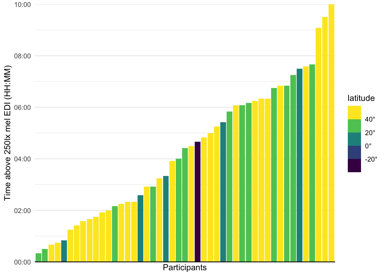
Time above threshold

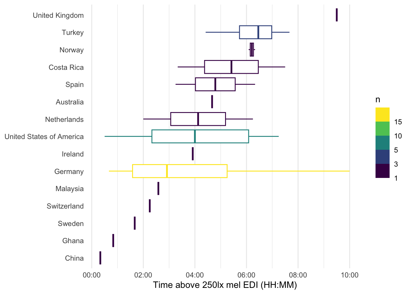
In this section we calculate the time above threshold for the single day of 22 September 2025 across latitude and country.

TAT250 <- 
light_data_ext |> 
  filter_Date(start = "2025-09-22", length = "1day") |> 
  fill(latitude, longitude, city, country, .direction = "downup") |> 
  dplyr::summarize(
    duration_above_threshold(
      MEDI, Datetime, threshold = 250, na.rm = TRUE,
      as.df = TRUE
    ),
    latitude = unique(latitude),
    longitude = unique(longitude),
    city = unique(city),
    country = unique(country)
  ) |> 
  mutate(n = n(), .by = country)

TAT250_plot <- function(value){
TAT250 |> 
  ggplot(aes(x= fct_reorder(Id, duration_above_250), y = duration_above_250))+
  geom_col(aes(fill = {{ value }})) +
  scale_fill_viridis_b(labels = \(x) paste0(x, "°"))+
  scale_y_time(labels = \(x) x |> as_datetime(tz = "UTC") |> format("%H:%M"),
               expand = FALSE) + 
  theme_minimal() +
  theme_sub_axis_x(text = element_blank(), line = element_line()) +
  theme_sub_panel(grid.major.x = element_blank())+
  labs(x = "Participants", y = "Time above 250lx mel EDI (HH:MM)")
}

# TAT250_plot(longitude) / (TAT250_plot(latitude) + ylim(c(10*3600, 0))) + plot_layout(axis = "collect", heights = c(1,0.05,1))

TAT250_plot(latitude)

ggsave("figures/Fig4_TAT250.png", width = 5, height = 2, scale = 1.5)

TAT250 |> 
  ggplot(aes(y= fct_reorder(country, duration_above_250), x = duration_above_250))+
  geom_boxplot(aes(col = n)) +
  scale_color_viridis_b(breaks = c(1, 3, 5, 10, 15))+
  scale_x_time(labels = \(x) x |> as_datetime(tz = "UTC") |> format("%H:%M")) + 
  theme_minimal() +
  # theme_sub_axis_x(text = element_blank(), line = element_line()) +
  theme_sub_panel(grid.major.y = element_blank())+
  labs(y = NULL, x = "Time above 250lx mel EDI (HH:MM)")

ggsave("figures/Fig5_TAT250_country.png", width = 4, height = 3, scale = 1.5)

Global perspectives

In this section we look at the global distribution of melanopic EDI, Time above 250lx, and the Dose of light.

Shade data

In this section we calculate day and night times around the globe. As we want to use this information for a looped visualization, we will set a slightly different cutoff and only collect 48 hours.

# Time window (UTC)
t_start <- ymd_hms("2025-09-21 12:00:00", tz = "UTC")
t_end   <- ymd_hms("2025-09-23 12:00:00", tz = "UTC")
# Step between frames (adjust to taste: "30 mins", "1 hour", etc.)
time_step <- "30 mins"

# Spatial grid resolution (degrees). 2° keeps things light; 1° looks smoother but is heavier.
lon_step <- 0.5
lat_step <- 0.5

# Darkness mapping: fully dark at civil twilight (-6°), linearly increasing from 0 to 1 as altitude goes 0 -> -6°.
dark_full_altitude <- -6 # degrees

# ---------- build lon/lat grid ----------
lons <- seq(-180, 180, by = lon_step)
lats <- seq(-90,  90,  by = lat_step)
grid <- expand.grid(lon = lons, lat = lats) |>
  as_tibble()

# ---------- time sequence ----------
times_utc <- seq(t_start, t_end, by = time_step)

# ---------- compute sun altitude for each (lon, lat, time) ----------
# We'll loop over time slices (efficient enough for this grid size),
# compute altitude (in radians from suncalc), convert to degrees,
# then map to a "darkness" alpha value.

compute_slice <- function(tt) {
  
  # build a data frame with the timestamp repeated for each grid point
  df <- data.frame(
    date = rep(tt, nrow(grid)),
    lat  = grid$lat,
    lon  = grid$lon
  )
  
  # call suncalc with a data frame instead of separate lat/lon vectors
  sp <- suncalc::getSunlightPosition(data = df, keep = c("altitude"))
  
  # altitude is returned in radians; convert to degrees
  alt_deg <- sp$altitude * 180 / pi
  
  # darkness mapping (same as before)
  darkness <- pmin(1, pmax(0, -alt_deg / 6))
  
  tibble(
    lon = grid$lon,
    lat = grid$lat,
    time = tt,
    alt_deg = alt_deg,
    darkness = darkness
  )
}

# Create the progress bar once
pb <- progress_bar$new(
  format = "Computing slices [:bar] :percent eta: :eta",
  total = length(times_utc), clear = FALSE, width = 70
)

shade_list <- vector("list", length(times_utc))

for (i in seq_along(times_utc)) {
  # Compute one time slice (without pb$tick() inside)
  shade_list[[i]] <- compute_slice(times_utc[[i]])
  # Now update the bar
  pb$tick()
}

shade_df <- dplyr::bind_rows(shade_list)

shade_df <- bind_rows(lapply(times_utc, compute_slice))

Melanopic EDI

Light data

light_data_globe <- 
light_data_ext |> 
    filter_Datetime(DatetimeUTC, start = t_start, end = t_end, tz = "UTC") |> 
    select(Id, DatetimeUTC, latitude, longitude, MEDI) |> 
    dplyr::mutate(lat2 = plyr::round_any(latitude, 12), 
           lon2 = plyr::round_any(longitude, 12)) |> 
    ungroup() |> 
    dplyr::summarize(
        .by = c(DatetimeUTC, lat2, lon2),
        lat = mean(latitude),
        lon = mean(longitude),
        MEDI = mean(MEDI, na.rm = TRUE),
        n = n()
    ) |> 
    rename(time = DatetimeUTC)

light_globe <- st_as_sf(light_data_globe, coords = c("lon", "lat"), crs = 4326)
light_proj <- st_transform(light_globe, crs = "+proj=eqc")

Plot

p <- 
  ggplot() +
  geom_sf(
    data = world_proj,
    fill = "grey",
    color = NA,
    size = 0.25,
    alpha = 0.5,
    show.legend = FALSE
  ) +
  geom_sf(data = tz_lines,
          colour = "deepskyblue3",
          alpha = 0.75,
          linewidth = 0.1) +
  geom_tile(
    data = shade_df,
    mapping = aes(x = lon, y = lat, alpha = darkness),
    fill = "black",
    width = lon_step, height = lat_step
  ) +
  geom_sf(
    data = light_proj,
    aes(size = n, fill = MEDI, colour = MEDI),
    alpha = 0.9,
    shape = 21,
    stroke = 0.2
  ) +
  # tile overlay for night shading (black with varying alpha)
  geom_sf_text(
    data = locations_proj,
    aes(label = n),
    size = 1.9,
    fontface = 2,
    color = "white",
    alpha = 0.75
  ) +
  scale_alpha(range = c(0, 0.6), limits = c(0, 1), guide = "none") +
  coord_sf(crs = 4326, expand = FALSE, xlim = c(-180, 180), ylim = c(-90, 90)) +
  # coord_sf(crs = 4326, xlim = c(-180, 180), ylim = c(-90, 90)) +
  labs(
    title = "{format(frame_time, '%Y-%m-%d %H:%M:%S', tz = 'UTC')} (UTC)",
    x = NULL, 
    y = NULL
  ) +
  guides(size = "none",
        )+
  labs(fill = "mel EDI (lx)", colour = "mel EDI (lx)")+
  scale_fill_viridis_b(trans = "symlog", breaks = c(0, 10^(0:5)),
                       labels = 
                         function(x) format(x, scientific = FALSE, big.mark = " "),
                       limits = c(0, 10^5)) +
  scale_colour_viridis_b(trans = "symlog", breaks = c(0, 10^(0:5)),
                       labels = 
                         function(x) format(x, scientific = FALSE, big.mark = " "),
                       limits = c(0, 10^5)) +
  scale_size_continuous(range = c(3, 7.5)) +
  theme_minimal(base_size = 13) +
  theme(
    panel.grid.major = element_line(size = 0.1, colour = "grey85"),
    panel.grid.minor = element_blank(),
    plot.title = element_text(face = "bold"),
    legend.text.align = 1,
    legend.text.position = "left",
    legend.position = "inside",
    legend.position.inside = c(0.1,0.35),
    legend.background = element_rect(fill = alpha("white", alpha = 0.25),
                                     colour = NA)
  ) +
  transition_time(time)

# Frame rate and dimensions
fps_out <- 10
width_px <- 1400
height_px <- 800

if(interactive()) {

anim <- animate(
  p,
  duration = 48*2,
  fps = fps_out,
  width = width_px,
  height = height_px,
  res = 150,
  renderer = magick_renderer(loop = TRUE)
)

out_file <- "figures/Fig6_melEDI_global.mp4"
image_write_video(anim, out_file, framerate = fps_out)
out_file <- "figures/Fig6_melEDI_global.gif"
image_write_gif(anim, out_file, delay = 1/fps_out)
}

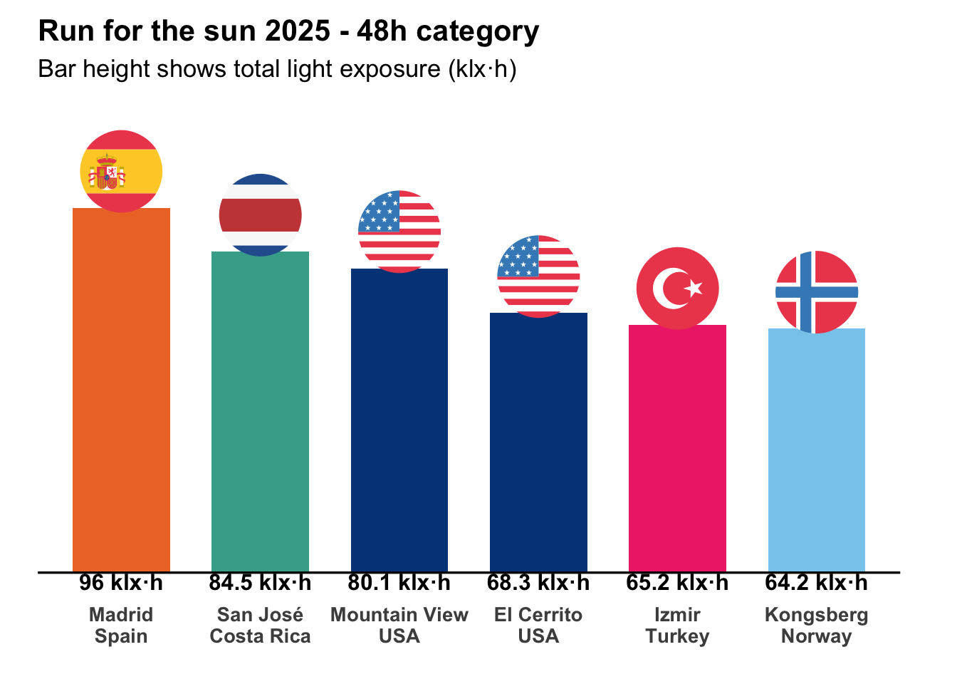
Race to the highest light dose

In this section we create an animated race to the highest light dose.

country_colors <- c(
  "Switzerland"              = "#CC3311",
  "Spain"                    = "#EE7733",
  "Germany"                  = "#332288",
  "Ghana"                    = "#117733",
  "Turkey"                   = "#EE3377",
  "Netherlands"              = "#0077BB",
  "China"                    = "#BB5566",
  "Malaysia"                 = "#33BBEE",
  "USA"                      = "#004488",
  "Norway"                   = "#88CCEE",
  "UK"                       = "#AA4499",
  "Ireland"                  = "#88AA55",
  "Sweden"                   = "#DDAA33",
  "Costa Rica"               = "#44AA99",
  "Australia"                = "#999933"
)

dose_race_data <- 
light_data_ext |>
  filter_Datetime(DatetimeUTC, start = t_start, end = t_end, tz = "UTC") |> 
  dplyr::filter(!travel_time_zone) |> 
  select(Id, DatetimeUTC, MEDI, type, setting_light, 
         city, country, latitude, longitude) |> 
  dplyr::rename(Datetime = DatetimeUTC) |>
  # aggregate_Datetime("12 hours") |> 
  dplyr::mutate(Dose = (MEDI/12),
                Dose = ifelse(is.na(Dose), 0, Dose),
                Dose = cumsum(Dose),
                Rando = runif(n(), 0, 0.01),
                Dose = Dose - first(Dose) + Rando,
                .after = MEDI) |> 
  group_by(Datetime) |> 
  dplyr::mutate(rank = rank(Dose),
                country = as.factor(country),
                country = case_match(country,
                  "United Kingdom" ~ "UK",
                  "United States of America" ~ "USA",
                  .default = country
                ),
                location = paste0(city, ", ", country)) |> 
  ungroup() 

dose_race <- 
dose_race_data |> 
  ggplot() +
  geom_col(aes(x=rank, y=Dose, group=Id, fill = country), 
           width = 0.8, position = "identity") +
  geom_text(aes(x=rank, y=Dose, 
                label= signif(round(Dose), 3), 
                group=Id), hjust= -0.25, size = 2) +
  geom_richtext(aes(x=rank, y=-1, 
                    label=ifelse(rank >= (44-5), glue("<b>{location}</b>"), location), 
                    group=Id), 
                fill = NA,
                label.color = NA,
                label.padding = unit(rep(0,4), "pt"),
                hjust= 1, size = 2) +
  theme_minimal() + 
  ylab('Light exposure (dose, lx·h)') +
  theme(axis.title.y = element_blank(),
        panel.grid.major.y = element_blank(),
        panel.grid.minor.y = element_blank(),
        axis.text.y = element_blank(),
        axis.ticks.y = element_blank(),
        plot.margin = unit(c(1,3,1,8), 'lines')) +
  guides(fill = "none")+
  scale_fill_manual(values = country_colors) +
  coord_flip(clip='off')

# dose_race + facet_grid(cols=vars(Datetime))

anim.plot <- 
  dose_race + 
  ggtitle("{format(frame_time, '%Y-%m-%d %H:%M:%S', tz = 'UTC')} (UTC)") +
  transition_time(Datetime) +
  view_follow()

# anim.plot
if(interactive()) {

anim2 <- animate(
  anim.plot,
  duration = 48*2,
  fps = fps_out,
  width = width_px,
  height = height_px,
  res = 150,
  renderer = magick_renderer()
)

out_file <- "figures/Fig7_Light_dose.mp4"

image_write_video(anim2, out_file, framerate = fps_out)

anim.plot <- 
  dose_race + 
  # ggtitle("{format(frame_time, '%Y-%m-%d %H:%M:%S', tz = 'UTC')} (UTC)") + 
  transition_time(Datetime) +
  view_follow()

anim2 <- animate(
  anim.plot,
  duration = 48*2,
  fps = fps_out,
  width = width_px/2,
  height = height_px,
  res = 150,
  renderer = magick_renderer()
)


out_file <- "figures/Fig7_Light_dose.gif"

image_write_gif(anim2, out_file, delay = 1/fps_out)

}

if(interactive()) {
  
  new_gif <- image_append(c(anim[1], anim2[1]))

  for(i in 2:(960)) {
    new_gif <- c(new_gif, image_append(c(anim[i], anim2[i])))
  }
  
  image_write_gif(new_gif,"figures/Fig7b_Light_dose.gif", 1/fps_out)
  image_write_video(new_gif,"figures/Fig7b_Light_dose.mp4", framerate = fps_out)

}

# Winners data
df <- tibble::tribble(
  ~rank, ~city,          ~country,                    ~score_klxh, ~iso2,
      1, "Madrid",       "Spain",                         96.0,    "es",
      2, "San José",     "Costa Rica",                    84.5,    "cr",
      3, "Mountain View","USA",                           80.1,    "us",
      4, "El Cerrito",   "USA",                           68.3,    "us",
      5, "Izmir",        "Turkey",                        65.2,    "tr",
      6, "Kongsberg",    "Norway",                        64.2,    "no"
) %>%
  mutate(
    label = paste0(city, "\n", country),
    # Order by rank (1 on the left)
    label = fct_reorder(label, rank)
  )

# Base plot: pedestals
p <- ggplot(df, aes(x = label, y = score_klxh, fill = country)) +
  geom_col(width = 0.7) +
  # Score labels on the pedestals
  geom_text(aes(label = paste0(score_klxh, " klx·h"), y = -6),
            vjust = -0.35, 
            size = 4.2, fontface = "bold") +
  geom_hline(yintercept = 0) +
  # Flags slightly above each pedestal top
  # ggflags wants numeric x; convert discrete x to numeric positions
  geom_flag(
    aes(x = as.numeric(label),
        y = score_klxh + max(score_klxh) * 0.10,
        country = iso2),
    size = 18
  ) +
  scale_fill_manual(values = country_colors) +
  labs(
    title = "Run for the sun 2025 - 48h category",
    subtitle = "Bar height shows total light exposure (klx·h)",
    x = NULL, y = NULL
  ) +
  coord_cartesian(ylim = c(0, max(df$score_klxh) * 1.25), clip = "off") +
  theme_minimal(base_size = 13) +
  theme(
    panel.grid.major = element_blank(),
    panel.grid.minor = element_blank(),
    axis.text.x = element_text(face = "bold"),
    plot.title = element_text(face = "bold"),
    axis.text.y = element_blank(),
    legend.position = "none",
    plot.margin = margin(10, 30, 20, 20)
  )

p

ggsave("figures/Fig8_pedestal.png", p, width = 7, height = 6)

Time zone travelers

In this section, we look at travelers across time zones

data_flights <- 
  data |> 
  filter(travel_time_zone == 1, !is.na(device_id), detailed_time_zone_changes_complete == 2) |> 
  select(device_id, record_id, travel_departure_time:longitude, tz_identifier_start:flight_no)

table_flights <- 
  data_flights |> 
  gt() |> 
  tab_style(locations = cells_column_labels(), style = cell_text(weight = "bold")) |> cols_align("left")
  
table_flights

Device ID	Record ID	Travel across time zones If yes, please list departure time zone(s):	Travel across time zones Arrival time zone(s):	Travel across time zones Approximate dates/time of travel:	City and country	Latitude	Longitude	TZ identifier (start)	Time start	TZ identifier (end)	Time start	Flight number
6275	35	Dublin	Madrid	6:00 am Dublin 7:00 am Madrid	Dublin (half) Madrid (half)	53,35	-6,26	Europe/Dublin	2025-09-22 06:03	Europe/Madrid	2025-09-22 09:04	FR10
4396	36	UTC+2	UTC+3	Between 13-14:20 on the 22nd. Time zone UTC+2.	Borås, Sweden and Helsinki, Finland	57,72 Borås; 60,17 Helsinki	12,94 Borås; 24,94 Helsinki	Europe/Stockholm	2025-09-22 13:06	Europe/Helsinki	2025-09-22 15:13	FIN864
6293	46	6:00 (UTC +1)	9:30 (UTC +2)	09/22/2025	MADRID	40°30′N	3°40′W	Europe/Dublin	2025-09-22 06:03	Europe/Madrid	2025-09-22 09:04	FR10

gtsave(table_flights, "tables/table_flights.png", vwidth = 1200)

file:////var/folders/9p/326_k3kx43qbn_cyl1rqfhb00000gn/T//RtmpQk3ZUL/file5ad93187c2b4.html screenshot completed

data_flights_cond <-
data_flights |> 
  select(Id = device_id, tz_identifier_start:flight_no) |> 
  dplyr::mutate(start = as_datetime(datetime_start),
                # start = force_tzs(start, tz_identifier_start, tzone_out = "UTC"),
                end = as_datetime(datetime_end) - dhours(1),
                # end = force_tzs(end, tz_identifier_end, tzone_out = "UTC"),
                Id = factor(Id)
                ) |> 
  select(-c(datetime_start, datetime_end)) |>
  group_by(Id)

light_data_ext |>
  add_states(data_flights_cond) |> 
  filter(travel_time_zone) |> 
  mutate(Id = fct_inseq(Id)) |> 
  gg_days(group = interaction(Id, consecutive_id(flight_no)),
          y.axis.label = "Melanopic EDI (lx)") |> 
  gg_state(setting_light, aes_fill = setting_light, alpha = 0.5) +
  aes(linewidth = !is.na(flight_no)) +
  scale_fill_manual(
    values = c(
      Bed = "darkgrey",
      `Non-wear` = "tomato",
      Indoors = "gold",
      Outdoors = "skyblue2",
      Mixed = "lightgreen"
    )
  ) + 
  scale_linewidth_manual(values = c(`TRUE` = 1, `FALSE` = 0.25)) +
  labs(fill = "Condition", linewidth = "Flighttime")

Scale for fill is already present.
Adding another scale for fill, which will replace the existing scale.

ggsave("figures/Fig3c_flyers.png", width = 6, height = 4, scale = 2)

# light_data_ext |> 
#   filter(travel_time_zone) |> 
#   add_states(data_flights_cond) |> 
#   mutate(Id = fct_inseq(Id)) |> 
#   ungroup() |> 
#   nest(.by = c(Id, latitude, longitude, tz_identifier)) |> 
#   mutate(data = list(data, latitude, longitude) |> pmap(\(x,y,z) add_photoperiod(x, c(y, z)))) |> 
#   unnest(data) |> 
#   group_by(Id) |> 
#   gg_days() |> 
#   gg_photoperiod()

light_data_ext |>
  add_states(data_flights_cond) |> 
  filter(travel_time_zone, !is.na(flight_no)) |> 
  gg_day(aes_col = Id,
          y.axis.label = "Melanopic EDI (lx)",
         alpha = 0.75) |> 
  gg_state(setting_mixed, aes_fill = setting_mixed, alpha = 0.25)+
  labs(color = "ID", fill = "Condition") +
    scale_fill_manual(
    values = c("lightgreen"
    )
    )

Scale for fill is already present.
Adding another scale for fill, which will replace the existing scale.

ggsave("figures/Fig3d_flyers.png", width = 4, height = 1.5, scale = 2)

Export for dashboard

In this section we export key data for the dashboard.

save(
     data_devices,
     events_complete,
     light_data_ext,
     histogram_plot,
     light_data_1day,
     timeline_plot,
     duration_tibble,
     duration_table,
     TAT250,
     file = "data/cleaned/dashboard.RData")