---
title: "Research Question 3"
subtitle: "Is personal light exposure related to participant characteristics?"
author: "Johannes Zauner"
format:
html:
toc: true
code-tools: true
code-link: true
page-layout: full
code-fold: show
---
## Preface
This document contains the analysis for Research Question 3, as defined in the [preregistration]( https://aspredicted.org/te3zw2.pdf).
> **Research Question 3**: \
Is personal light exposure related to participant characteristics?
>
> *H8*: Duration, exposure-history, and level-based metrics of personal light exposure are significantly associated with personal light sensitivity (VLSQ-8)
>
> *H9*: Timing-based metrics of personal light exposure are significantly associated with chronotype.
>
> *H10*: Personal light exposure metrics depend on age and sex
>
> *H11*: Personal light exposure patterns depend on sex
>
## Setup
In this section, we load in the [preprocessed](data_preparation.qmd) and [prepared](metric_preparation.qmd) data, site data, and load required packages.
```{r}
#| message: false
#| warning: false
#| code-summary: Code cell - Setup
library(tidyverse)
library(melidosData)
library(LightLogR)
library(mgcv)
library(lme4)
library(performance)
library(cowplot)
library(ggridges)
library(ggtext)
library(sjPlot)
library(broom)
library(itsadug)
library(gratia)
library(emmeans)
library(patchwork)
library(rlang)
library(broom.mixed)
library(gt)
library(performance)
library(glmmTMB)
library(gghighlight)
library(gtsummary)
source("scripts/fitting.R")
source("scripts/summaries.R")
source("scripts/RQ2_specific.R")
```
```{r}
#| message: false
#| file-name: Load data
load("data/metrics_glasses.RData")
load("data/preprocessed_glasses_2.RData")
metrics <- metrics_glasses
hourly_data <-  light_glasses_processed2
H8 <- "Hypothesis: Duration, exposure-history, and level-based metrics of personal light exposure are significantly associated with personal light sensitivity (VLSQ-8)."
H9 <- "Hypothesis: Timing-based metrics of personal light exposure are significantly associated with chronotype."
H10 <- "Hypothesis: Personal light exposure metrics depend on age and sex."
H11 <- "Hypothesis: Personal light exposure patterns depend on sex."
sig.level <- 0.05

#for chest:
# load("data/metrics_chest.RData")
# metrics <- metrics_chest
# melidos_cities <- melidos_cities[names(melidos_cities)!="MPI"]
```
## Hypothesis 8
### Details
Hypothesis 3 states:
> Duration, exposure-history, and level-based metrics of personal light exposure are significantly associated with personal light sensitivity (VLSQ-8)
*Type of model:* GLMM
*Base formula:* $\text{metric} \sim \text{VLSQ-8}*\text{Site} + (1|\text{Participant})$
*Notes:*
- Site was sum-coded, so as to calculate an average effect of site
- Error family depends on the metric
*Specific formulas:*
- $\text{mel EDI} \sim \text{Site} + (1|\text{Site}:\text{Participant})$ (Null-model)
- $\text{mel EDI} \sim \text{VLSQ-8} + \text{Site} + (1|\text{Site}:\text{Participant})$ (Null-model interaction)
- $\text{mel EDI} \sim \text{VLSQ-8} + (1|\text{Participant})$ (Null-model site)
*False-discovery-rate correction:*
- 9 metrics with one confirmatory analysis: n=9
- For sites (interaction), n=9
### Preparation
```{r}
#| filename: Load VLSQ-8 data
vlsq8 <- load_data("vlsq8") |> flatten_data()
```
```{r}
#| code-summary: Code cell - Model setup based on distribution
model_tbl <- tibble::tribble(
    ~name, ~engine, ~ response, ~family,
    "interdaily_stability", "lm", "qlogis(metric)", gaussian(),
    "intradaily_variability", "lm", "metric", gaussian(),
    "Mean", "lmer", "log_zero_inflated(metric)", gaussian(),
    "dose", "lmer", "log_zero_inflated(metric)", gaussian(),
    "MDER", "lmer", "metric", gaussian(),
    "darkest_10h_mean", "lmer", "log_zero_inflated(metric)", gaussian(),
    "brightest_10h_mean", "lmer", "log_zero_inflated(metric)", gaussian(),
    "duration_above_1000", "glmmTMB", "metric", tweedie(link = "log"),
    "duration_above_250", "lmer", NA, gaussian(),
    "duration_below_10", "lmer", NA, gaussian(),
    "duration_below_1", "lmer", NA, gaussian(),
    "duration_above_250_wake", "glmmTMB", "metric", tweedie(link = "log"),
    "duration_below_10_pre-sleep", "glmmTMB", "metric", tweedie(link = "log"),
    "duration_below_1_sleep", "glmmTMB", "metric", tweedie(link = "log"),
    "period_above_250", "lmer", "log_zero_inflated(metric)", gaussian(),
    "brightest_10h_midpoint", "lmer", "metric", gaussian(),
    "brightest_10h_onset", "lmer", NA, gaussian(),
    "brightest_10h_offset", "lmer", NA, gaussian(),
    "darkest_10h_midpoint", "lmer", "metric", gaussian(),
    "darkest_10h_onset", "lmer", NA, gaussian(),
    "darkest_10h_offset", "lmer", NA, gaussian(),
    "mean_timing_above_250", "lmer", "metric", gaussian(),
    "first_timing_above_250", "lmer", "metric", gaussian(),
    "last_timing_above_250", "lmer", "metric", gaussian()
  )
```
```{r}
#| code-summary: Code cell - Formula setup for inference
H8_data <-
  metrics |>
  filter(metric_type %in% c("duration", "exposure history", "level")) |>
  filter_out(name == "duration_above_250") |>
  mutate(
    H8_1 = "~ site*VLSQ8 + (1|Id)",
    H8_0 = "~ site + (1|Id)",
    H8_ni = "~ site + VLSQ8 + (1|Id)",
    H8_ns = "~ VLSQ8 + (1|Id)",
         ) |>
  left_join(model_tbl, by = "name")

H8_formulas <-  names(H8_data) |> subset(grepl("H8_", names(H8_data)))

H8_data <-
  H8_data |> relocate(all_of(H8_formulas), .after = family)
H8_fdr_n <- H8_data |> filter(!is.na(response)) |> nrow()
```
```{r}
H8_data <-
  H8_data |>
  mutate(data = data |> map(\(x) x |> left_join(vlsq8, by = c("site", "Id"))))
```
```{r}
#| echo: false
H8_data |>
  select(-data) |>
  filter(!is.na(response)) |>
  arrange(metric_type, name) |>
  mutate(family = map(family, 1),
         rowname = seq_along(1:length(name))) |>
  group_by(metric_type) |>
  gt() |>
  cols_label_with(fn = \(x) x |> str_to_title() |> str_replace_all("_", " ")) |>
  sub_missing(missing_text = "") |>
  sub_values(values = "NULL", replacement = "") |>
  fmt(name, fns = \(x) x |> str_to_title() |>  str_replace_all("_", " ")) |>
  sub_values(values = "MDER", replacement = "MDER") |>
  tab_header("Hypothesis 8: metric model specifications",
             subtitle = H8) |>
  tab_footnote("Confirmatory analysis will use a p-value correction through the false-discovery rate for n=9 comparisons") |>
  tab_footnote("These are the models used for the confirmatory analysis. Each H1 1 and H1 0 pair are compaired with likelihood-ratio tests to determine whether site is meaningful", locations = cells_column_labels(c(H8_1, H8_0))) |>
  tab_footnote("These are the models used for exploratory analyses. Models are compared with all sensible combinations of hierarchical effects", locations = cells_column_labels(c(H8_ni, H8_ns)))
```
```{r}
#| code-summary: Code cell - Formula creation
H8_data <-
  H8_data |>
  mutate(across(all_of(H8_formulas),
                \(x) map2(x, response, \(y,z) make_formula(z, y))
                )
         )
```
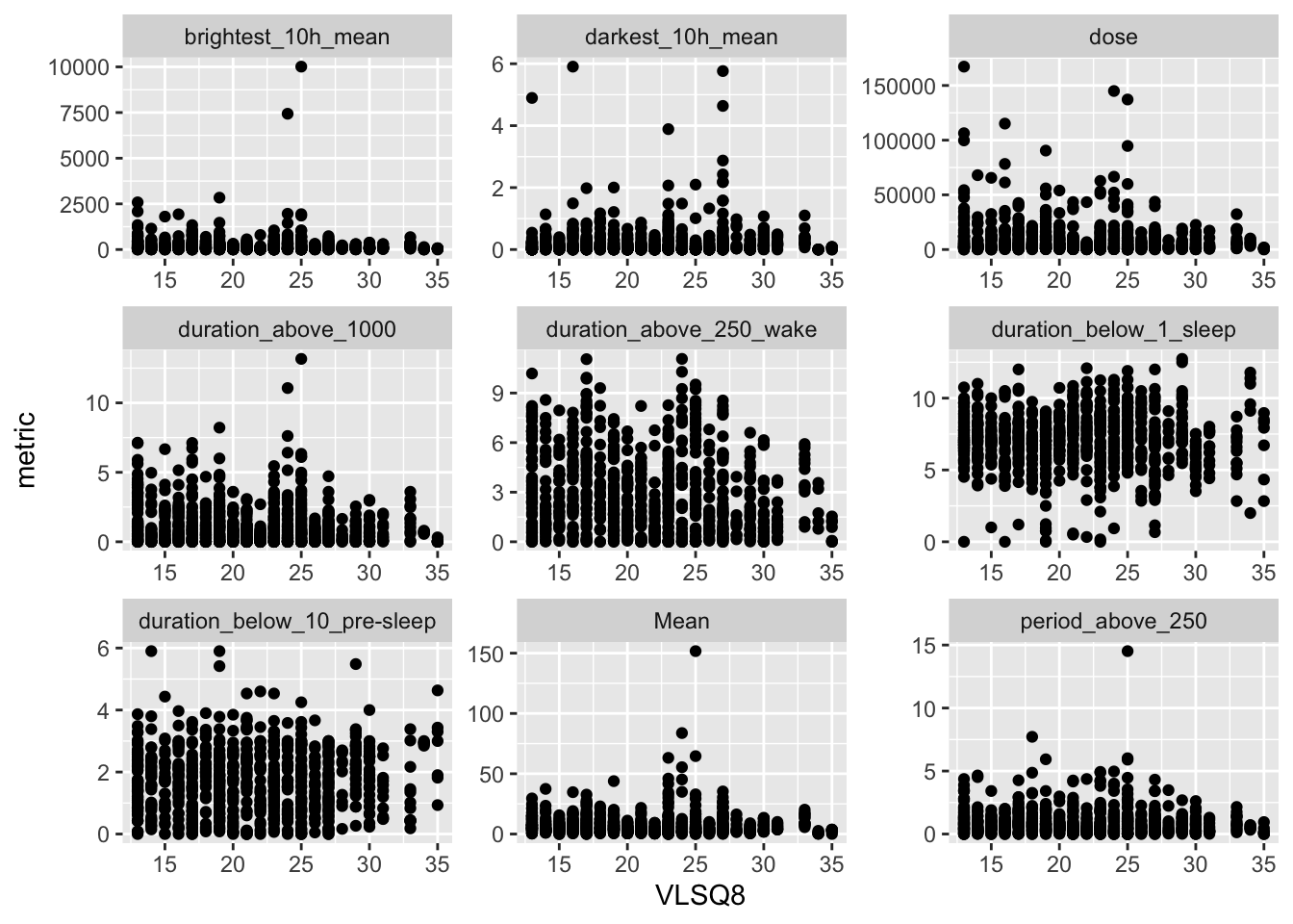
```{r}
H8_data |>
  select(name, data) |>
  unnest(data) |>
  ggplot(aes(x = VLSQ8, y = metric)) +
  geom_point() +
  facet_wrap(~name, scales = "free")
```
### Analysis
#### Fit models
```{r}
#| code-summary: Code cell - Model fit
#| message: false
H8_data <-
  H8_data |>
  mutate(
    across(all_of(H8_formulas),
           \(x) pmap(list(data, x, engine, family), fit_model),
           .names = "{.col}_model")
    )
```
Model diagnostics are omitted here. We checked in RQ1 for sensible base models
### Model comparisons
```{r}
#| code-summary: Code cell - Model comparisons
#| message: false
H8_data <-
  H8_data |>
  mutate(
    H8_1_comp = map2(H8_0_model, H8_1_model, model_anova),
    H8_1_p = map2(H8_1_comp, engine, model_comp_p, n = H8_fdr_n) |> list_c(),
    H8_1_sig = H8_1_p <= sig.level,

    H8_i_comp = map2(H8_ni_model, H8_1_model, model_anova),
    H8_i_p = map2(H8_i_comp, engine, model_comp_p, n = H8_fdr_n) |> list_c(),
    H8_i_sig = H8_i_p <= sig.level,

    H8_s_comp = map2(H8_ns_model, H8_ni_model, model_anova),
    H8_s_p = map2(H8_s_comp, engine, model_comp_p, n = H8_fdr_n) |> list_c(),
    H8_s_sig = H8_s_p <= sig.level,
  )
```
```{r}
H8_tab <-
H8_data |>
  select(metric_type, name, H8_1_p, H8_1_sig) |>
  mutate(H8_1_p = style_pvalue(H8_1_p)) |>
  gt() |>
  tab_header(
    "H8: Model results",
    subtitle = H8
  )
```
```{r}
H8_tab
gtsave(H8_tab, "tables/H8.png", vwidth = 1200)
gtsave(H8_tab, "tables/H8.docx", vwidth = 1200)
```
### Interpretation
None of the light exposure metrics are significantly associated with VLSQ-8 scores
## Hypothesis 9
### Details
Hypothesis 9 states:
> Timing-based metrics of personal light exposure are significantly associated with chronotype.
*Type of model:* GLMM
*Base formula:* $\text{metric} \sim \text{Chronotype}*\text{Site} + (1|\text{Participant})$
*Notes:*
- Site was sum-coded, so as to calculate an average effect of site
- Chronotype is operationalized through the MCTQ-score $msf_{sc}$ (Mid-sleep on free days. Sleep corrected)
- Error family depends on the metric
*Specific formulas:*
- $\text{mel EDI} \sim \text{Site} + (1|\text{Site}:\text{Participant})$ (Null-model)
- $\text{mel EDI} \sim \text{Chronotype} + \text{Site} + (1|\text{Site}:\text{Participant})$ (Null-model interaction)
- $\text{mel EDI} \sim \text{Chronotype} + (1|\text{Participant})$ (Null-model site)
*False-discovery-rate correction:*
- 5 metrics with one confirmatory analysis: n=5
- For sites (interaction), n=9
### Preparation
```{r}
#| filename: Load chronotype data
ct <- load_data("chronotype") |> flatten_data()
ct$msf_sc |> range(na.rm = TRUE) |> hms::as_hms()
ct <- ct |> mutate(msf_sc = as.numeric(msf_sc)/3600)
```
Since all msf_sc values are after midnight, we will use linear modelling instead of circular.
```{r}
#| code-summary: Code cell - Formula setup for inference
H9_data <-
  metrics |>
  filter(metric_type %in% c("timing")) |>
  filter_out(str_detect(name, "onset|offset")) |>
  mutate(
    H9_1 = "~ site*msf_sc + (1|Id)",
    H9_0 = "~ site + (1|Id)",
    H9_00 = "~ 1 + (1|Id)",
    H9_ni = "~ site + msf_sc + (1|Id)",
    H9_ns = "~ msf_sc + (1|Id)",
         ) |>
  left_join(model_tbl, by = "name")

H9_formulas <-  names(H9_data) |> subset(grepl("H9_", names(H9_data)))

H9_data <-
  H9_data |> relocate(all_of(H9_formulas), .after = family)
H9_fdr_n <- H9_data |> filter(!is.na(response)) |> nrow()
```
```{r}
H9_data <-
  H9_data |>
  mutate(data = data |> map(\(x) x |> left_join(ct, by = c("site", "Id")) |>
                              drop_na(msf_sc)))
```
```{r}
#| echo: false
H9_data |>
  select(-data) |>
  filter(!is.na(response)) |>
  arrange(metric_type, name) |>
  mutate(family = map(family, 1),
         rowname = seq_along(1:length(name))) |>
  group_by(metric_type) |>
  gt() |>
  cols_label_with(fn = \(x) x |> str_to_title() |> str_replace_all("_", " ")) |>
  sub_missing(missing_text = "") |>
  sub_values(values = "NULL", replacement = "") |>
  fmt(name, fns = \(x) x |> str_to_title() |>  str_replace_all("_", " ")) |>
  sub_values(values = "MDER", replacement = "MDER") |>
  tab_header("Hypothesis 9: metric model specifications",
             subtitle = H9) |>
  tab_footnote("Confirmatory analysis will use a p-value correction through the false-discovery rate for n=5 comparisons") |>
  tab_footnote("These are the models used for the confirmatory analysis. Each H1 1 and H1 0 pair are compaired with likelihood-ratio tests to determine whether site is meaningful", locations = cells_column_labels(c(H9_ni, H9_00))) |>
  tab_footnote("These are the models used for exploratory analyses. Models are compared with all sensible combinations of hierarchical effects", locations = cells_column_labels(c(H9_1, H9_ns, H9_0)))
```
```{r}
#| code-summary: Code cell - Formula creation
H9_data <-
  H9_data |>
  mutate(across(all_of(H9_formulas),
                \(x) map2(x, response, \(y,z) make_formula(z, y))
                )
         )
```
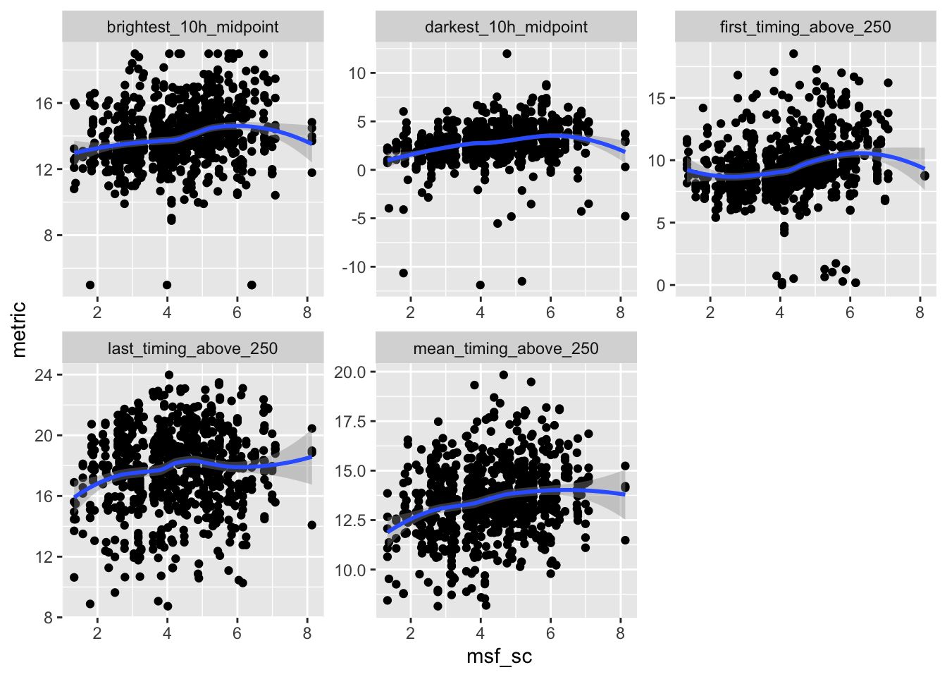
```{r}
H9_data |>
  select(name, data) |>
  unnest(data) |>
  ggplot(aes(x = msf_sc, y = metric)) +
  geom_point() +
  facet_wrap(~name, scales = "free") +
  geom_smooth()
```
### Analysis
#### Fit models
```{r}
#| code-summary: Code cell - Model fit
#| message: false
H9_data <-
  H9_data |>
  mutate(
    across(all_of(H9_formulas),
           \(x) pmap(list(data, x, engine, family), fit_model),
           .names = "{.col}_model")
    )
```
Model diagnostics are omitted here. We checked in RQ1 for sensible base models
```{r}
#| code-summary: Code cell - Model comparisons
#| message: false
H9_data <-
  H9_data |>
  mutate(
    H9_1_comp = map2(H9_00_model, H9_ns_model, model_anova),
    H9_1_p = map2(H9_1_comp, engine, model_comp_p, n = H9_fdr_n) |> list_c(),
    H9_1_sig = H9_1_p <= sig.level,

    H9_i_comp = map2(H9_ni_model, H9_1_model, model_anova),
    H9_i_p = map2(H9_i_comp, engine, model_comp_p, n = H9_fdr_n) |> list_c(),
    H9_i_sig = H9_i_p <= sig.level,

    H9_s_comp = map2(H9_ns_model, H9_ni_model, model_anova),
    H9_s_p = map2(H9_s_comp, engine, model_comp_p, n = H9_fdr_n) |> list_c(),
    H9_s_sig = H9_s_p <= sig.level,

    H9_model = pmap(
      list(H9_1_sig, H9_i_sig, H9_s_sig, H9_00_model, H9_0_model, H9_ns_model, H9_ni_model, H9_1_model),
      \(sig1, sig2, sig3, model00, model_site, model_ct, model_both, model_interaction) {
        if(all(sig1, sig2, sig3)) {
          model <- model_interaction
        } else if(all(sig1, sig3) & !sig2) {
            model <- model_both
        } else if(sig1 & !sig2 & !sig3) {
            model <- model_ct
        } else if(!sig1 & sig3 & !sig2) {
            model <- model_site
          } else model <- model00
          model
      }
      ),

    marginals = map(H9_ns_model, \(x) emtrends(x, ~ msf_sc, var = "msf_sc")),
    marginals = map2(H9_1_sig, marginals,
                     \(sig, marginal) {
                        if(sig) return(marginal |> as.tibble()) else return(tibble(msf_sc = NA))
                          }
    )
  )
```
```{r}
H9_data <-
H9_data |>
  mutate(
    H9_r2 = pmap(list(H9_ns_model, data, family, response), r2_helper),
    H9_marginal = map_dbl(H9_r2, \(x) x$R2_marginal),
    H9_marginal = ifelse(H9_1_sig, H9_marginal, NA)
  )
# |> pull(H9_r2)
```
#### Basic table
```{r}
H9_tab <-
H9_data |>
  select(
    metric_type, name, H9_1_sig, H9_1_p, marginals, H9_marginal
  ) |>
  unnest(marginals) |>
  gt() |>
  fmt_number() |>
    sub_missing(H9_marginal) |>
  fmt(H9_1_p, fns = style_pvalue) |>
  cols_merge(
    c(msf_sc.trend, SE, lower.CL, upper.CL),
    pattern = "<<**{1}** ±{2} ({3} - {4})>>"
  ) |>
  fmt(name, fns = \(x) x |> str_replace_all("_", " ") |> str_to_sentence()) |>
  as.data.frame() |>
  gt() |>

  tab_style(style = cell_text(weight = "bold"),
            locations = cells_body(H9_1_p, H9_1_sig == "TRUE")) |>
  cols_hide(c(H9_1_sig, df, msf_sc, metric_type, SE, lower.CL, upper.CL)) |>
  cols_label(
    H9_1_p = "p-value",
    msf_sc.trend = md("$MSF_{sc}$"),
    name = "Metric",
    H9_marginal = md("$R^2_{marginal}$")
  ) |>
  fmt_markdown(msf_sc.trend) |>
  tab_header(
    "H9: Model results",
    subtitle = H9
  ) |>
  tab_footnote(
    "p-value adjustment for n=5 model comparisons with FDR correction",
    locations = cells_column_labels(H9_1_p)
  ) |>
  sub_missing()
```
```{r}
H9_tab
H9_tab |> gtsave("tables/H9.png")
```
#### Visualization
```{r}
#| fig-width: 10
#| fig-height: 5
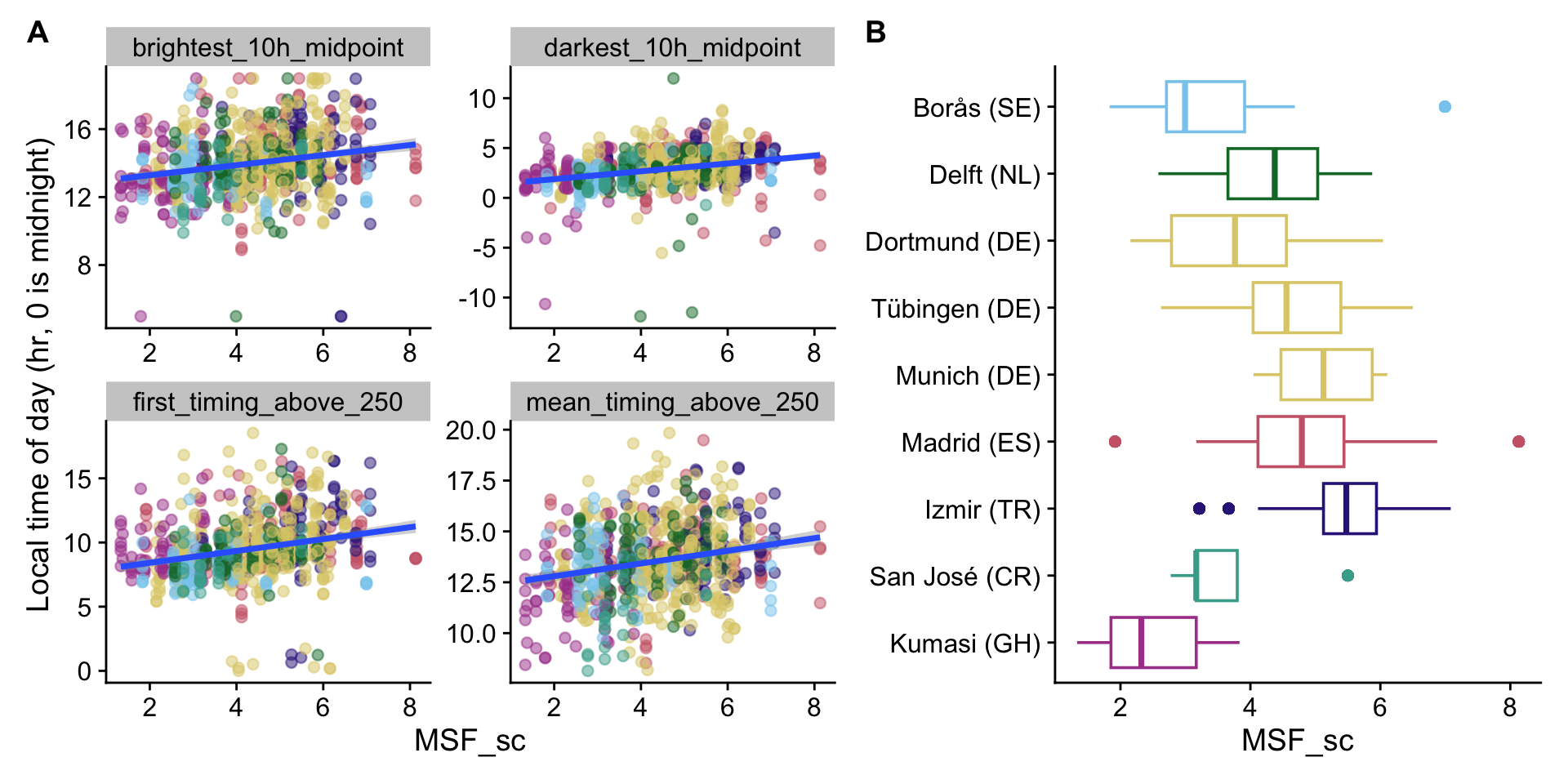
H9_plot1 <-
H9_data |>
select(name, data) |>
unnest(data) |>
site_conv_mutate(rev = FALSE) |>
filter_out(name == "last_timing_above_250") |>
ggplot(aes(x = msf_sc, y = metric)) +
geom_point(aes(color = site), alpha = 0.5) +
facet_wrap(~name, scales = "free") +
guides(color = "none") +
theme_cowplot() +
labs(y = "Local time of day (hr, 0 is midnight)", x = "MSF_sc") +
geom_smooth(method = "lm") +
scale_color_manual(values = melidos_colors)
H9_plot2 <-
H9_data |>
select(name, data) |>
unnest(data) |>
site_conv_mutate(rev = TRUE) |>
filter_out(name == "last_timing_above_250") |>
ggplot(aes(x = msf_sc, y = site, color = site)) +
geom_boxplot() +
theme_cowplot() +
guides(color = "none") +
labs(y = NULL, x = "MSF_sc") +
scale_color_manual(values = melidos_colors)
H9_plot1 + H9_plot2 + plot_layout(widths = c(3,2)) + plot_annotation(tag_levels = "A")
ggsave("figures/Fig7.pdf", width = 10, height = 5)
ggsave("figures/Fig7.png", width = 10, height = 5)
```
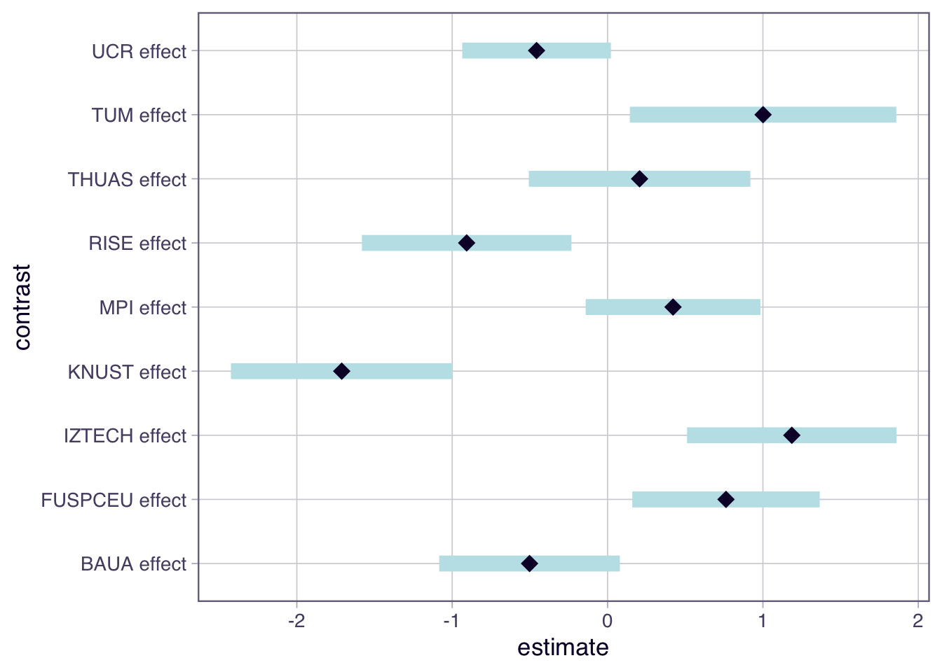
```{r}
lm(msf_sc ~ site, data = ct, contrasts = list(site = "contr.sum")) |> drop1(test = "Chisq")
lm(msf_sc ~ site, data = ct, contrasts = list(site = "contr.sum")) |>
  emmeans(~ site) |> contrast() |> plot()
lm(msf_sc ~ photoperiod + site, data = H9_data$data[[1]]) |> drop1(test = "Chisq")
lm(msf_sc ~ photoperiod + site, data = H9_data$data[[1]]) |> summary()
lm(msf_sc ~ photoperiod + site, data = H9_data$data[[1]]) |>
  emmeans(~ site) |> contrast()
```
### Interpretation
- Chronotype is an important dependency timing-based metrics. Per one hour later MSF_sc, participants experience important aspects of the day about 0.31 to 0.44 hours later in the day, including the brightest and darkest 10h midpoint, mean and first timing about 250lx melanopic EDI. The last timing above 250 lx melanopic EDI was not significant
- Chronotype is significantly different between sites
## Hypothesis 10
### Details
Hypothesis 10 states:
> Personal light exposure metrics depend on age and sex
*Type of model:* GLMM
*Base formulas:*
- $\text{mel EDI} \sim \text{sex/age} + \text{Site} + (1|\text{Participant})$
*Notes:*
- Site was sum-coded, so as to calculate an average effect of site
- Error family depends on the metric
*Specific formulas:*
- $\text{mel EDI} \sim \text{Site} + (1|\text{Participant})$ (Null-model)
- $\text{metric} \sim \text{sex/age}*\text{Site} + (1|\text{Participant})$ (Interaction-model)
*False-discovery-rate correction:*
- 17 metrics with one confirmatory analysis times 2 variables: n=34
- For sites (interaction), n=9
### Preparation
```{r}
#| filename: load demographics
demographics <- load_data("demographics") |> flatten_data()
```
```{r}
lm(age ~ site, data = demographics) |> emmeans(~ site) |> contrast()
lm(age ~ site, data = demographics) |> drop1(test = "Chisq")
demographics |> ggplot(aes(x = site, y = age)) + geom_boxplot()
```
```{r}
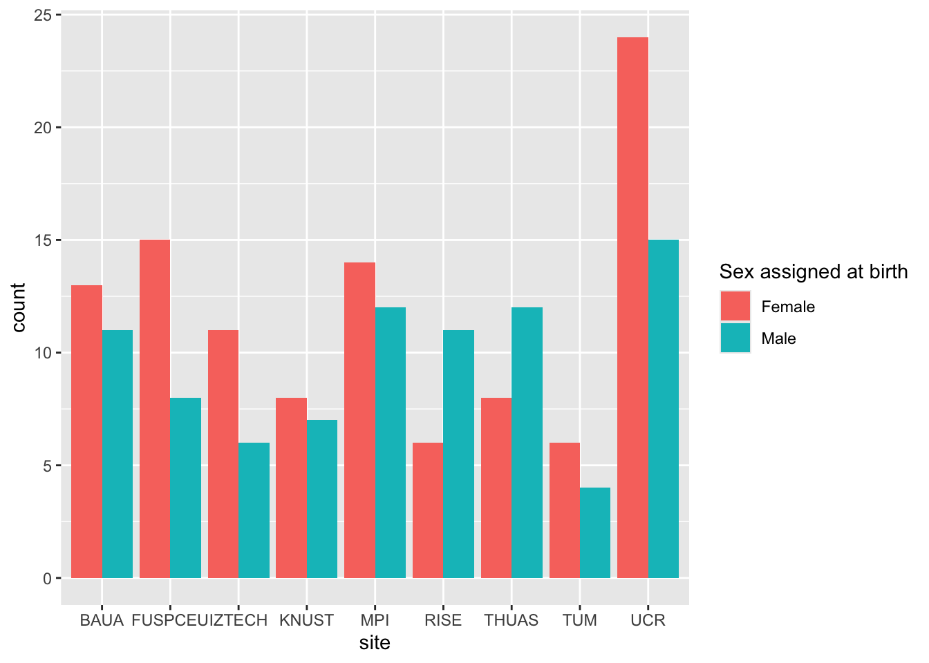
glm(sex ~ site, data = demographics, family = binomial()) |> emmeans(~ site) |> contrast()
glm(sex ~ site, data = demographics, family = binomial()) |> drop1(test = "Chisq")
demographics |> ggplot(aes(x = site, fill = sex)) + geom_bar(position = position_dodge())
```
> age shows significant differences between sites, sex does not
```{r}
#| code-summary: Code cell - Formula setup for inference
H10_data <-
  metrics |>
  left_join(model_tbl, by = "name") |>
  filter_out(is.na(response)) |>
  mutate(
    H10_1a = "~ site + age + (1|Id)",
    H10_1s = "~ site + sex + (1|Id)",
    H10_0 = "~ site + (1|Id)",
    H10_a = "~ age + (1|Id)",
    H10_00 = "~ 1 + (1|Id)",
    H10_ia = "~ site*age + (1|Id)",
    H10_is = "~ site*sex + (1|Id)",
    across(H10_1a:H10_is,
           \(x) ifelse(engine == "lm", str_remove(x, " \\+ \\(1\\|Id\\)"), x)
             ),
         )

H10_formulas <-  names(H10_data) |> subset(grepl("H10_", names(H10_data)))

H10_data <-
  H10_data |> relocate(all_of(H10_formulas), .after = family)
H10_fdr_n <- H10_data |> filter(!is.na(response)) |> nrow() *2
```
```{r}
#| echo: false
H10_data |>
  select(-data) |>
  filter(!is.na(response)) |>
  arrange(metric_type, name) |>
  mutate(family = map(family, 1),
         rowname = seq_along(1:length(name))) |>
  group_by(metric_type) |>
  gt() |>
  cols_label_with(fn = \(x) x |> str_to_title() |> str_replace_all("_", " ")) |>
  sub_missing(missing_text = "") |>
  sub_values(values = "NULL", replacement = "") |>
  fmt(name, fns = \(x) x |> str_to_title() |>  str_replace_all("_", " ")) |>
  sub_values(values = "MDER", replacement = "MDER") |>
  tab_header("Hypothesis 9: metric model specifications",
             subtitle = H10) |>
  tab_footnote("Confirmatory analysis will use a p-value correction through the false-discovery rate for n=34 comparisons") |>
  tab_footnote("These are the models used for the confirmatory analysis. Each H1 1 and H1 0 pair are compaired with likelihood-ratio tests to determine whether site is meaningful", locations = cells_column_labels(c(H10_1s, H10_1a, H10_0))) |>
  tab_footnote("These are the models used for exploratory analyses. Models are compared with all sensible combinations of hierarchical effects", locations = cells_column_labels(c(H10_is, H10_ia, H10_00)))
```
```{r}
#| code-summary: Code cell - Formula creation
H10_data <-
  H10_data |>
  mutate(across(all_of(H10_formulas),
                \(x) map2(x, response, \(y,z) make_formula(z, y))
                )
         )
```
```{r}
#| fig-height: 8
#| fig-width: 15
H10_data |>
  select(name, data) |>
  unnest(data) |>
  ggplot(aes(x = age, y = metric)) +
  geom_point() +
  facet_wrap(~name, scales = "free") +
  geom_smooth()
```
```{r}
#| fig-height: 8
#| fig-width: 15
H10_data |>
select(name, data) |>
unnest(data) |>
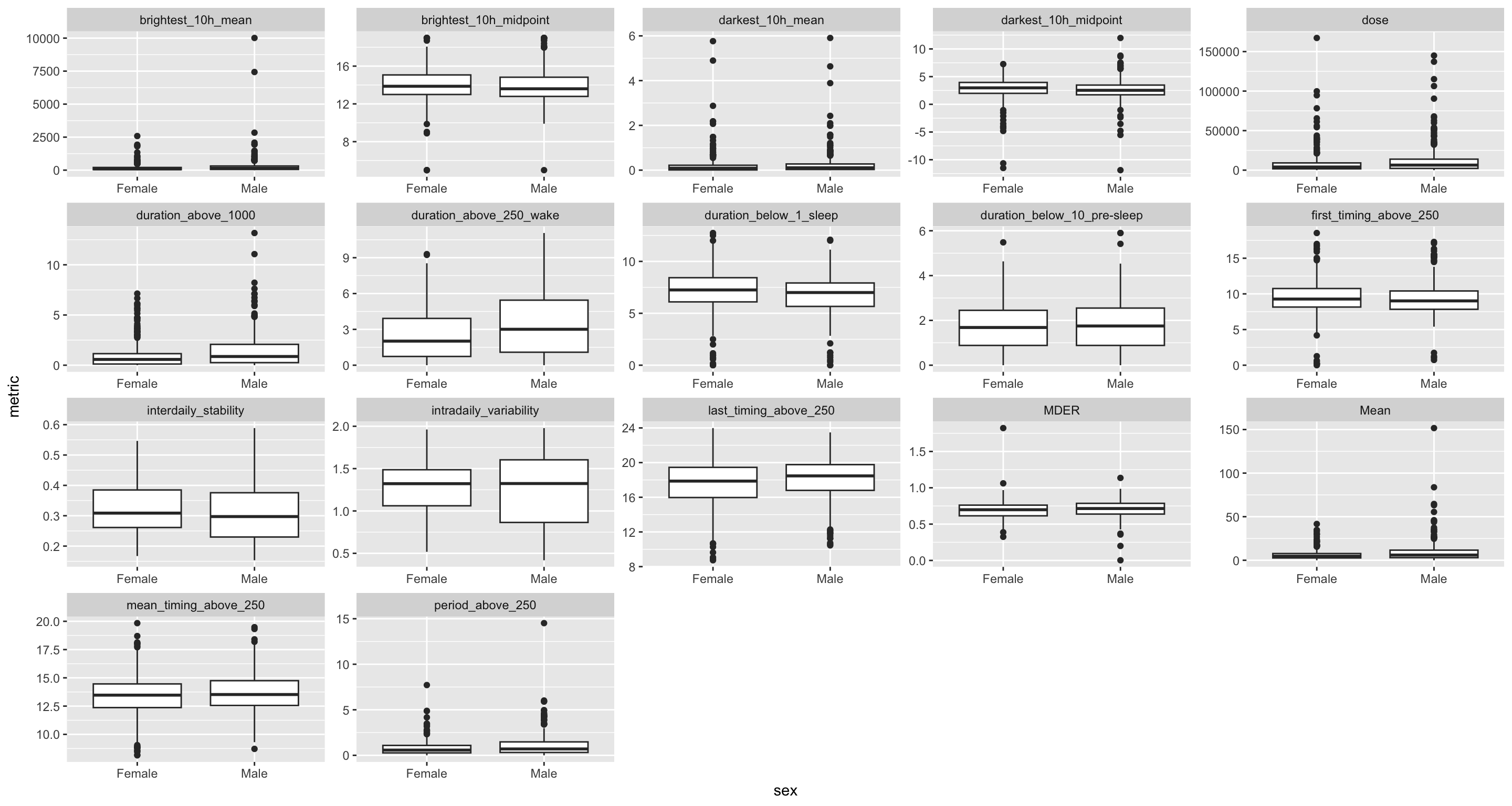
ggplot(aes(x = sex, y = metric)) +
geom_boxplot() +
facet_wrap(~name, scales = "free") +
geom_smooth()
```
### Analysis
#### Fit models
```{r}
#| code-summary: Code cell - Model fit
#| message: false
H10_data <-
  H10_data |>
  mutate(
    across(all_of(H10_formulas),
           \(x) pmap(list(data, x, engine, family), fit_model),
           .names = "{.col}_model")
    )
```
Model diagnostics are omitted here. We checked in RQ1 for sensible base models
```{r}
#| code-summary: Code cell - Model comparisons
#| message: false
H10_data <-
  H10_data |>
  mutate(
    H10_1s_comp = map2(H10_0_model, H10_1s_model, model_anova),
    H10_1s_p = map2(H10_1s_comp, engine, model_comp_p, n = H10_fdr_n) |> list_c(),
    H10_1s_sig = H10_1s_p <= sig.level,

    H10_1a_comp = map2(H10_0_model, H10_1a_model, model_anova),
    H10_1a_p = map2(H10_1a_comp, engine, model_comp_p, n = H10_fdr_n) |> list_c(),
    H10_1a_sig = H10_1a_p <= sig.level,

    H10_ia_comp = map2(H10_1a_model, H10_ia_model, model_anova),
    H10_ia_p = map2(H10_ia_comp, engine, model_comp_p, n = H10_fdr_n) |> list_c(),
    H10_ia_sig = H10_ia_p <= sig.level,

    marginals = map(H10_1a_model, \(x) emtrends(x, ~ age, var = "age") |> as.tibble()),
  )
```
```{r}
H10_data |>
  select(metric_type, name, ends_with(c("_p", "_sig"))) |>
  gt() |>
  fmt(where(is.numeric), fns = style_pvalue) |>
  tab_style(cell_text(weight = "bold"),
            locations = cells_body(H10_1a_p, H10_1a_sig)) |>
  cols_hide(ends_with("_sig")) |>
  tab_header("H10: Overall model results",
             subtitle = H10) |>
  tab_footnote("H10_1s_p: p-values for sex, H10_1a_p: p-values for age, H10_ia_p: p-values for interaction of age with site. p-values where adjusted with FDR method and n=34", locations = cells_column_labels(ends_with("_p")))
```
After the initial testing, only a single model was significant. The next table summarizes this model
```{r}
H10_data <-
H10_data |>
  mutate(
    H10_r2 = pmap(list(H10_a_model, data, family, response), r2_helper),
    H10_marginal = map_dbl(H10_r2, \(x) x$R2_marginal),
    H10_marginal = ifelse(H10_1a_sig, H10_marginal, NA)
  )
# |> pull(H10_r2)
```
#### Basic table
```{r}
H10_tab <-
H10_data |>
  filter(H10_1a_sig) |>
  select(
    metric_type, name, H10_1a_sig, H10_1a_p, marginals, H10_marginal
  ) |>
  unnest(marginals) |>
  gt() |>
  fmt_number(decimals = 3) |>
    sub_missing(H10_marginal) |>
  fmt(H10_1a_p, fns = style_pvalue) |>
  cols_merge(
    c(age.trend, SE, asymp.LCL, asymp.UCL),
    pattern = "<<**{1}** ±{2} ({3} - {4})>>"
  ) |>
  fmt(name, fns = \(x) x |> str_replace_all("_", " ") |> str_to_sentence()) |>
  as.data.frame() |>
  gt() |>

  tab_style(style = cell_text(weight = "bold"),
            locations = cells_body(H10_1a_p, H10_1a_sig == "TRUE")) |>
  cols_hide(c(H10_1a_sig, df, age, metric_type, SE, asymp.LCL, asymp.UCL)) |>
  cols_label(
    H10_1a_p = "p-value",
    age.trend = "Age",
    name = "Metric",
    H10_marginal = md("$R^2_{marginal}$")
  ) |>
  fmt_markdown(age.trend) |>
  tab_header(
    "H10: Model results",
    subtitle = H10
  ) |>
  tab_footnote(
    "p-value adjustment for n=34 model comparisons with FDR correction",
    locations = cells_column_labels(H10_1a_p)
  ) |>
  sub_missing()
```
```{r}
H10_tab
H10_tab |> gtsave("tables/H10.png")
```
#### Visualization
```{r}
#| fig-width: 10
#| fig-height: 5
H10_plot1 <-
H10_data |>
select(name, data) |>
unnest(data) |>
site_conv_mutate(rev = FALSE) |>
filter(name == "duration_above_1000") |>
ggplot(aes(x = age, y = metric)) +
geom_point(aes(color = site), alpha = 0.5) +
facet_wrap(~name, scales = "free") +
guides(color = "none") +
theme_cowplot() +
labs(y = "Local time of day (hr)", x = "Age (yrs)") +
geom_smooth(method = "lm") +
scale_color_manual(values = melidos_colors)
H10_plot2 <-
H10_data |>
select(name, data) |>
unnest(data) |>
site_conv_mutate(rev = TRUE) |>
filter_out(name == "last_timing_above_250") |>
ggplot(aes(x = age, y = site, color = site)) +
geom_boxplot() +
theme_cowplot() +
guides(color = "none") +
labs(y = NULL, x = "Age (yrs)") +
scale_color_manual(values = melidos_colors)
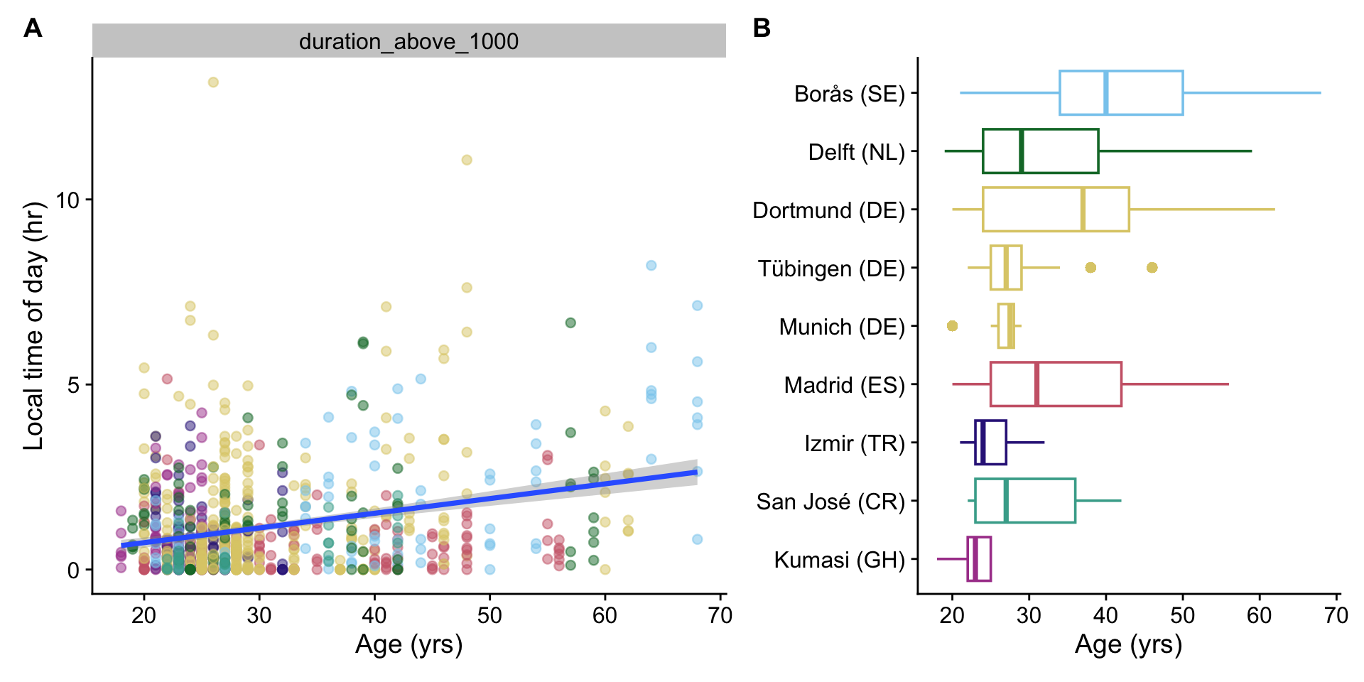
H10_plot1 + H10_plot2 + plot_layout(widths = c(3,2)) + plot_annotation(tag_levels = "A")
ggsave("figures/Fig8.pdf", width = 10, height = 5)
ggsave("figures/Fig8.png", width = 10, height = 5)
```
### Interpretation
Overall, there are no strong connections between melanopic EDI based metrics and `age` or `sex` in these datasets. The execption is a strong dependency of `age` with `Duration above 1000 lx melanopic EDI`, where for every 10 years of age, about 15 minutes more daily time above 1000 lx is reached. This effect is marginally relevant, with about 7.4% of variance explained.
## Hypothesis 11
Hypothesis 11 states:
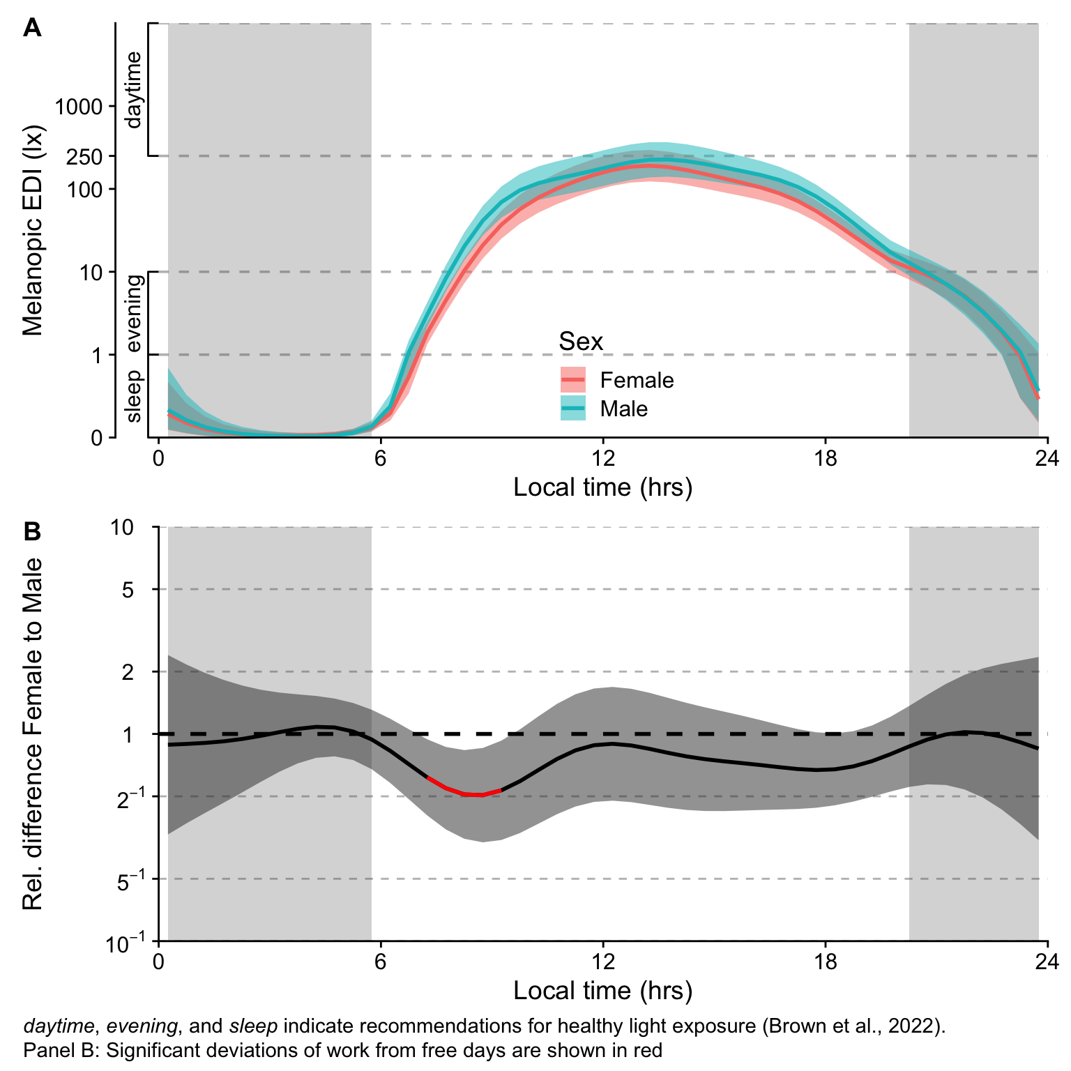
> Personal light exposure patterns depend on sex
*Type of model:* HGAM (Hierarchical GAM)
*Base formula:* $\text{melanopic EDI} \sim s(\text{Time}) + s(\text{Time}, \text{Sex}) + s(\text{Time}, \text{Site}) + s(\text{Time}, \text{Participant})$
*Additional notes:*
- Site effects are modelled with the `sz` basis, that allows for the most identifiable modelling of parametric differences
- Participant effects are modelled with the `fs` basis, which models the participant-effects as random smooths
- melanopic EDI is scaled with `log_zero_inflated()` before model fitting.
- The modle is based on the result from H2
*Specific formulas:*
- $\text{melanopic EDI} \sim s(\text{Time}) + s(\text{Time}, \text{Site}) + s(\text{Time}, \text{Participant})$ (comparison to the base formula)
*False-discovery-rate correction:*
1 (there is only one main comparison that tests the effect of site)
### Preparation
```{r}
#| filename: Load prepared data
load("data/metrics_separate_glasses.RData")
load("data/preprocessed_glasses_2.RData")

metric_participanthour <-
  metric_glasses_participanthour |>
  add_Time_col() |>
  ungroup() |>
  mutate(Time = as.numeric(Time)/3600 + 0.25,
         across(c(site, Id, sleep, State.Brown, wear, photoperiod.state),
                fct),
         Date = factor(Date),
         Id_date = interaction(Id, Date),
         lzMEDI = log_zero_inflated(MEDI),
         photoperiod = (dusk - dawn) |> as.numeric()
  ) |>
  group_by(Id) |>
  mutate(AR.start = ifelse(row_number() == 1, TRUE, FALSE)) |>
  ungroup() |>
  left_join(demographics, by = c("site", "Id")) |>
  mutate(across(c(site, Id), fct))
```
```{r}
#| filename: Overview plot of the data (median with IQR)
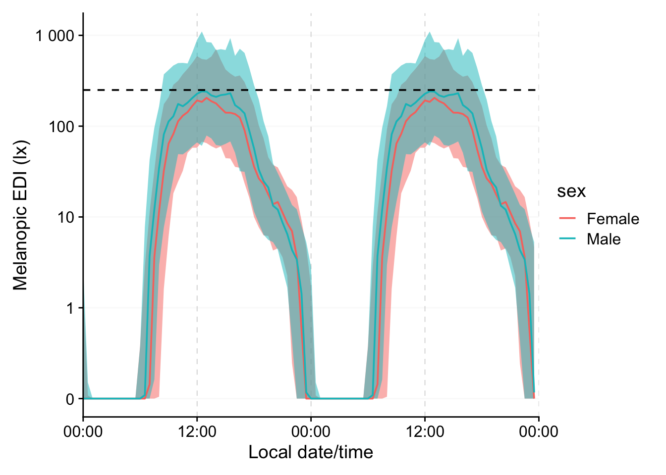
metric_participanthour |>
group_by(sex) |>
aggregate_Date(
date.handler = \(x) ymd("2025-01-01"),
numeric.handler = \(x) median(x, na.rm = TRUE),
p75 = quantile(MEDI, p=0.75, na.rm = TRUE),
p25 = quantile(MEDI, p=0.25, na.rm = TRUE)
) |>
gg_doubleplot(geom = "blank", jco_color = FALSE, facetting = FALSE,
x.axis.breaks.repeat = ~Datetime_breaks(.x, by = "12 hours", shift =
lubridate::duration(0, "hours"))) +
geom_ribbon(aes(ymin = p25, ymax = p75, fill = sex), alpha = 0.5) +
geom_line(aes(color = sex)) +
geom_hline(yintercept = 250, linetype = "dashed") +
# facet_wrap(~sex, scales = "free_x") +
guides(fill = "none") +
theme(panel.spacing = unit(2, "lines"))
```
```{r}
#| filename: H11 formulas
H11_form_1 <- lzMEDI ~ s(Time, k = 12) + s(Time, photoperiod.state, bs = "sz", k=12) + s(Time, sex, bs = "sz", k = 12) + s(Time, site, bs = "sz", k = 12) + s(Time, Id, bs = "fs") + s(Id_date, bs = "re")
H11_form_0 <- lzMEDI ~ s(Time, k = 12) + s(Time, photoperiod.state, bs = "sz", k=12) + s(Time, site, bs = "sz", k = 12) + s(Time, Id, bs = "fs") + s(Id_date, bs = "re")
```
### Analysis
#### Base model (H11_1)
```{r}
#| filename: Main model
H11_model_1 <-
  bam(H11_form_1,
      data = metric_participanthour,
      discrete = TRUE,
      method = "fREML",
      nthreads = 10
      )

r1 <- start_value_rho(H11_model_1,
                      plot=TRUE)
H11_model_1 <-
bam(H11_form_1,
data = metric_participanthour,
discrete = TRUE,
method = "fREML",
nthreads = 10,
rho = r1,
AR.start = AR.start
)
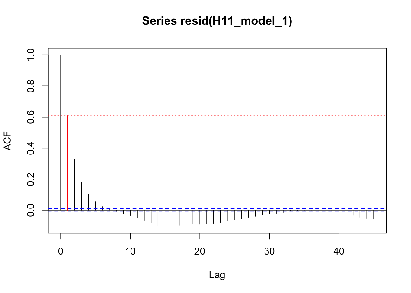
acf_resid(H11_model_1, split_pred = "AR.start")
H11_summary_1 <- summary(H11_model_1)
H11_summary_1
H11_model_1 |> glance()
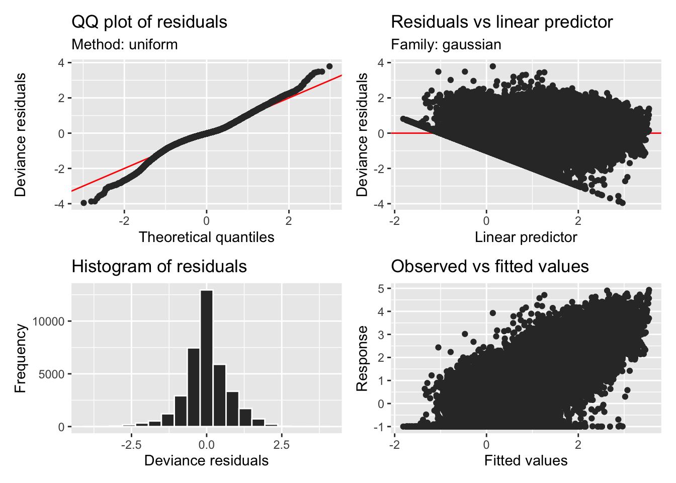
H11_model_1 |> appraise()
```
```{r}
#| filename: Variance explained
Xp <- predict(H11_model_1, type = "terms")
variance <- apply(Xp, 2, var)
cor(Xp)
H11_R2 <- (variance/sum(variance)) |> enframe(value = "R2", name = "parameter")
H11_R2
```
#### Null model (H11_0)
```{r}
#| filename: Null model
H11_model_0 <-
  bam(H11_form_0,
      data = metric_participanthour,
      discrete = TRUE,
      method = "fREML",
      nthreads = 8
      )

r1 <- start_value_rho(H11_model_0,
                      plot=TRUE)
H11_model_0 <-
bam(H11_form_0,
data = metric_participanthour,
discrete = TRUE,
method = "fREML",
nthreads = 10,
rho = r1,
AR.start = AR.start
)
acf_resid(H11_model_0, split_pred = "AR.start")
H11_summary_0 <- summary(H11_model_0)
H11_summary_0
H11_model_0 |> glance()
H11_model_0 |> appraise()
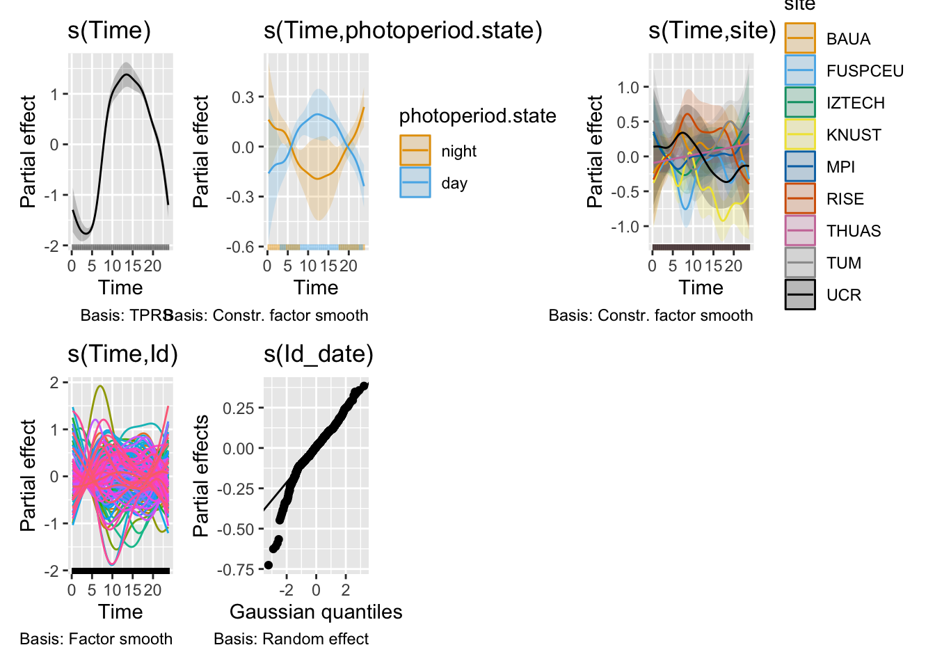
H11_model_0 |> draw()
```
#### Model comparison
```{r}
H11_AICs <- AIC(H11_model_1, H11_model_0)
H11_AICs |> as_tibble(rownames = "model") |> gt()
```
> While sex only explains very little of the overall structure (<1% of variance explained), is has a ∆AIC >2 and will thus be included
#### Model visualization
```{r}
#| filename: prepare lightsource model H11 plot
H11_data <-
H11_model_1 |>
  conditional_values(
    condition = list(Time = seq(0.25, 23.75, by = 0.5), "sex", "photoperiod.state"),
    exclude = c("s(Time,Id)", "s(Id_date)", "s(Time,site)")
    ) |>
  mutate(across(c(.fitted, .lower_ci, .upper_ci),
                exp_zero_inflated)
  )

H11_data <-
metric_participanthour |>
  Datetime2Time() |>
  group_by(sex, Time) |>
  summarize(
    .groups = "drop_last",
    dawn = dawn |> as.numeric() |> mean(na.rm = TRUE)/3600,
    dusk = dusk |> as.numeric() |> mean(na.rm = TRUE)/3600,
    n = n()
  ) |>
  mutate(
    photoperiod.state = ifelse(between(Time, dawn, dusk), "day", "night")
  ) |>
  select(-c(dawn, dusk)) |>
  left_join(H11_data, by = c("sex", "Time", "photoperiod.state"))

H11_data_phot <-
H11_data |>
  number_states(photoperiod.state) |>
  filter(photoperiod.state == "night") |>
  group_by(sex, photoperiod.state.count) |>
  summarize(xmin = min(Time),
            xmax = max(Time),
            .groups = "drop_last") |>
  mutate(across(c(xmin, xmax), \(x) replace_values(x,
                                                   0.5 ~ 0,
                                                   23.5 ~ 24)))
```
```{r}
#| filename: Visualize lightsource model H11
#| fig-height: 5
#| fig-width: 14
source("scripts/Brown_bracket.R")
H11_pred <-
H11_data |>
ggplot(aes()) +
map(c(1,10,250, 10^4),
\(x) geom_hline(aes(yintercept = x),
col = "grey", linetype = "dashed")
) +
geom_rect(data = H11_data_phot |> filter(sex == "Female"),
aes(xmin = xmin, ymin = -Inf, ymax = Inf, xmax = xmax),
alpha = 0.25, inherit.aes = FALSE) +
geom_ribbon(aes(x = Time, ymin = .lower_ci,
ymax = .upper_ci, fill = sex), alpha = 0.5) +
geom_line(aes(x = Time, y = .fitted,
col = sex), linewidth = 1) +
# scale_fill_manual(values = act_colors) +
# scale_color_manual(values = act_colors) +
theme_cowplot() +
scale_y_continuous(trans = "symlog", breaks = c(0,1,10,100,250, 1000)) +
scale_x_continuous(breaks = seq(0, 24, by = 6)) +
coord_cartesian(xlim = c(0,24), ylim = c(0,10^4), expand = FALSE) +
labs(y = "Melanopic EDI (lx)", x = "Local time (hrs)", fill = "Sex", col = "Sex") +
# facet_wrap(~sex, nrow = 1) +
guides( y = guide_axis_stack(Brown_bracket, "axis")) +
# gghighlight(
# label_key = sex,
# label_params = list(x = 12, y = 4.5, force = 0, hjust = 0.5)
# ) +
# geom_text(aes(label = paste0("|", n, "|"), x = Time, y = 7000), size = rel(1.5)) +
theme_sub_strip(background = element_blank(),
text = element_blank()) +
theme(panel.spacing = unit(1, "lines"),
plot.caption = element_textbox_simple(),
legend.position = "inside",
legend.position.inside = c(0.45, 0.15)
)
# labs(caption = Brown_caption)
H11_pred
```
```{r}
df <- H11_model_1$model |> distinct(Time, .keep_all = TRUE)
H11_termplot <-
difference_sz(H11_model_1,
              df,
              "Time", "sex", "Female", "Male",
              "s(Time,sex)",
              exclude = c("s(Time,site)", "s(Time,Id)", "s(Id_date)"),
              unconditional = FALSE,
              level = 0.95
  ) |>
    mutate(
         signif = lower > 0 | upper < 0,
         signif_id = consecutive_id(signif)) |>
  ggplot(aes()) +
  map(c(log10(c(0.1, 0.2, 0.5, 2, 5, 10))),
      \(x) geom_hline(yintercept = x, linewidth = 0.5, col = "grey", linetype = 2)) +
  geom_rect(data = H11_data_phot |> filter(sex == "Female"),
            aes(xmin = xmin, ymin = -Inf, ymax = Inf, xmax = xmax),
            alpha = 0.25, inherit.aes = FALSE) +
  geom_ribbon(aes(x = Time, ymin = lower, ymax = upper), alpha = 0.5) +
  geom_hline(yintercept = 0, linewidth = 1, linetype = 2) +
  geom_line(aes(x = Time, y = diff),
            linewidth = 1) +
  geom_line(data = \(x) filter(x, signif),
            aes(x = Time, y = diff, group = signif_id),
            col = "red", linewidth = 1) +
    theme_cowplot() +
  scale_y_continuous(labels = expression(10^-1, 5^-1, 2^-1, "1  ", "2  ", "5  ", "10  "),
                     breaks = log10(c(0.1, 0.2, 0.5, 1, 2, 5, 10)))+
  scale_x_continuous(breaks = seq(0, 24, by = 6)) +
  coord_cartesian(xlim = c(0,24), expand = FALSE) +
  guides(fill = "none") +
  labs(y = "Rel. difference Female to Male", x = "Local time (hrs)") +
  theme_sub_strip(background = element_blank(),
                  text = element_blank()) +
  theme(panel.spacing = unit(1, "lines"),
        plot.caption = element_textbox_simple())
```
```{r}
#| fig-height: 8
#| fig-width: 8
#| filename: Combination of partial plots H11

H11_pred / H11_termplot +
  plot_annotation(tag_levels = "A",
                  caption = paste(Brown_caption,
                                  "Panel B: Significant deviations of work from free days are shown in red", sep = "<br>"),
                  theme =
                    theme(plot.caption = element_textbox_simple(size = rel(1))
                          )
                  )
ggsave("figures/Fig13.pdf", height = 8, width = 7.3)
ggsave("figures/Fig13.png", height = 8, width = 7.3)
```
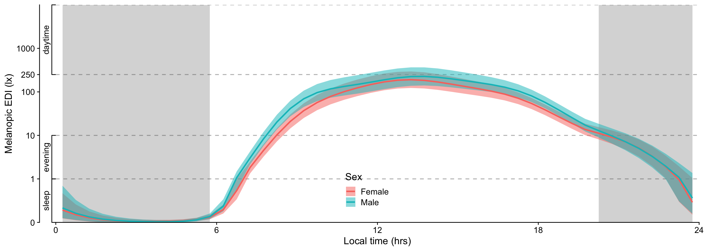
### Interpretation
- Sex is a minor differentiator in terms of melanopic stimulus, that explanes less than 1% of the variance. The only significant difference between the sexes is a lower value during the morning for females compared to males. This phase lasts about 2 hours and has a peak difference of about factor 2.
### Testing for other drivers
```{r}
mHLEA <- load_data("lightexposurediary") |> flatten_data()
mHLEA_labels <-
  mHLEA|> extract_labels() |>
  enframe() |>
  filter(str_detect(name, "act_")) |>
  mutate(name = name |> str_remove("act_"))

hourly_data <-
  metric_participanthour #|>
  # aggregate_Datetime(
  #   "1 hour",
  #   type = "floor",
  #   numeric.handler = \(x) x |> mean(na.rm = TRUE),
  #   geo.MEDI = MEDI |> log_zero_inflated() |> mean(na.rm = TRUE) |> exp_zero_inflated()
  # )|>
  # add_Date_col(group.by = TRUE) |>
  # mutate(static = all(MEDI == MEDI[1])) |>
  # filter_out(static) |>
  # select(-static) |>
  # ungroup(Date)

hourly_data <-
  hourly_data |>
  group_by(site, Id, Date) |>
  add_states(mHLEA |> mutate(Date = factor(Date)))

hourly_data2 <-
  hourly_data |>
  group_by(site, lightsource_primary) |>
  mutate(n = n(),
         lightsource_primary = lightsource_primary |>
           replace_when((n < 20 ) ~ NA)
           ) |>
  group_by(lightsource_primary) |>
  mutate(n = n(),
         lightsource_primary = lightsource_primary |>
           replace_when((n < 200 ) ~ NA,
                        lightsource_primary == "Light entering from outside during sleep" ~ NA),
         site = factor(site)
           )

activity_data <-
hourly_data2 |>
  ungroup() |>
  select(site, sex, Id, Time, lzMEDI, Id_date, photoperiod, photoperiod.state, starts_with("act_"), Datetime, lightsource_primary) |>
  pivot_longer(cols = starts_with("act_"), names_to = "activity", names_prefix = "act_", values_to = "value") |>
  filter(value, !is.na(lzMEDI)) |>
  distinct(.keep_all = TRUE, site, sex, Time, Id, Datetime, photoperiod.state, activity) |>
  select(-value) |>
  mutate(
    Id = factor(Id)
  ) |>
    group_by(Id) |>
  mutate(AR.start = ifelse(row_number() == 1, TRUE, FALSE)) |>
  ungroup()

activity_data <-
  activity_data |>
  mutate(activity =
           fct(activity) |>
           fct_collapse(outdoor = c("free_outdoor", "working_outdoor", "road_open")) |>
           fct_recode(NULL = "other") |>
           fct_relevel("home")
         )
```
```{r}
#| filename: H11 formulas
H11_form_1b <- lzMEDI ~ s(Time, k = 12) + s(Time, photoperiod.state, bs = "sz", k=12) + s(Time, activity, bs = "sz", k = 12) + s(Time, site, bs = "sz", k = 12) + s(Time, Id, bs = "fs") + s(Id_date, bs = "re")
H11_form_2 <- lzMEDI ~ s(Time, k = 12) + s(Time, photoperiod.state, bs = "sz", k=12) + s(Time, sex, bs = "sz", k = 12) + s(Time, activity, bs = "sz", k = 12) + s(Time, site, bs = "sz", k = 12) + s(Time, Id, bs = "fs") + s(Id_date, bs = "re")
```
```{r}
#| filename: Main model
H11_model_1b <-
  bam(H11_form_1b,
      data = activity_data,
      discrete = TRUE,
      method = "fREML",
      nthreads = 10
      )

r1 <- start_value_rho(H11_model_1b,
                      plot=TRUE)
H11_model_1b <-
bam(H11_form_1b,
data = activity_data,
discrete = TRUE,
method = "fREML",
nthreads = 10,
rho = r1,
AR.start = AR.start
)
acf_resid(H11_model_1b, split_pred = "AR.start")
```
```{r}
#| filename: Activity model
H11_model_2 <-
  bam(H11_form_2,
      data = activity_data,
      discrete = TRUE,
      method = "fREML",
      nthreads = 10
      )

r1 <- start_value_rho(H11_model_2,
                      plot=TRUE)
H11_model_2 <-
bam(H11_form_2,
data = activity_data,
discrete = TRUE,
method = "fREML",
nthreads = 10,
rho = r1,
AR.start = AR.start
)
acf_resid(H11_model_2, split_pred = "AR.start")
```
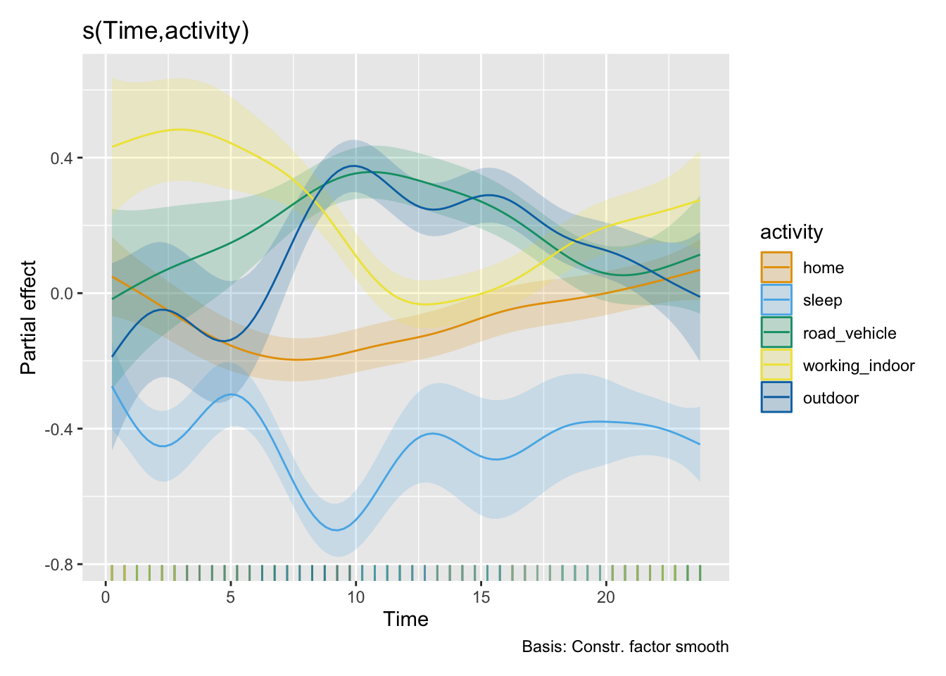
```{r}
# H11_model_1b |> draw(select = "s(Time,sex)")
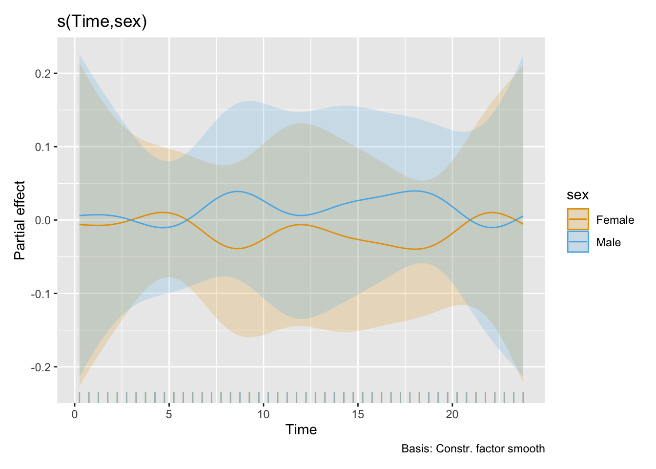
H11_model_2 |> draw(select = "s(Time,sex)")
H11_model_2 |> draw(select = "s(Time,activity)")
AIC(H11_model_1b, H11_model_2)
```
## Session Info
```{r}
sessionInfo()
```