---
title: "Personal light exposure: Metric preparation"
subtitle: "Individual, behavioural, and environmental determinants of personal light exposure in daily life: a multi-country wearable and experience-sampling study"
format:
html:
code-tools: true
code-link: true
---
## Preface
This script works off [the data preprocessing](data_preparation.qmd), to produce one dataframe containing all metrics in numeric form, ready for analysis.
### How metrics must be interpreted
- Timing and duration-based metrics are converted to decimal-hours.
- In the case of timing they mean decimal-hours from midnight.
- The `darkest_10h` are centered on midnight, i.e., values before midnight are negative.
- `mean` value metrics used a geometric mean (with `log_zero_inflated()`).
For a single, unnested dataframe of metrics execute:
```
metrics_glasses |> unnest(data)
```
## Setup
```{r}
#| message: false
#| warning: false
#| filename: Setup
library(tidyverse)
library(melidosData)
library(LightLogR)
library(mgcv)
library(readxl)
library(lme4)
library(performance)
library(cowplot)
library(ggridges)
library(downlit)
library(xml2)
```
```{r}
#| message: false
#| filename: Load data
load("data/metrics_separate_glasses.RData")
load("data/metrics_separate_chest.RData")
load("data/preprocessed_glasses_2.RData")
load("data/preprocessed_chest_2.RData")
demographics <- load_data("demographics") |> flatten_data()
```
## Preparation
### Context
```{r}
#| filename: Prepare photoperiods
photoperiod_daily <-
light_glasses_processed2 |>
  group_by(site, Id, Date) |>
  summarize(photoperiod = mean(photoperiod, na.rm = TRUE) |> as.numeric(),
            .groups = "drop_last")

photoperiod_participant <-
light_glasses_processed2 |>
  group_by(site, Id) |>
  summarize(photoperiod = mean(photoperiod, na.rm = TRUE) |> as.numeric(),
            .groups = "drop_last")

photoperiod_daily_chest <-
light_chest_processed2 |>
  group_by(site, Id, Date) |>
  summarize(photoperiod = mean(photoperiod, na.rm = TRUE) |> as.numeric(),
            .groups = "drop_last")

photoperiod_participant_chest <-
light_chest_processed2 |>
  group_by(site, Id) |>
  summarize(photoperiod = mean(photoperiod, na.rm = TRUE) |> as.numeric(),
            .groups = "drop_last")
```
```{r}
#| filename: Prepare contextual info
demographics <-
  demographics |>
  select(site, Id, age, sex, gender, employment_status)

context <-
  tibble(site = names(melidos_cities),
         country = unname(melidos_countries),
         tz = unname(melidos_tzs),
         city = unname(melidos_cities),
         ) |>
  left_join(
    melidos_coordinates |> map(enframe) |> list_rbind(names_to = "site") |> pivot_wider() |> rename(lat = `1`, lon = `2`),
    by = "site"
  )

demographics <-
  demographics |>
  left_join(context, by = join_by("site"))
```
### Metrics
In this section, we will combine all the metrics into one data-frame
```{r}
#| filename: Prepare participant metrics
metrics_glasses <-
metric_glasses_participant |>
  left_join(demographics, by = c("site", "Id")) |>
  left_join(photoperiod_participant, by = c("site", "Id")) |>
  pivot_longer(c(interdaily_stability, intradaily_variability), names_to = "name", values_to = "metric") |>
  ungroup() |>
  nest(.by = name) |>
  mutate(type = "participant")

metrics_chest <-
metric_chest_participant |>
  left_join(demographics, by = c("site", "Id")) |>
  left_join(photoperiod_participant_chest, by = c("site", "Id")) |>
  pivot_longer(c(interdaily_stability, intradaily_variability), names_to = "name", values_to = "metric") |>
  ungroup() |>
  nest(.by = name) |>
  mutate(type = "participant")
```
```{r}
#| filename: Prepare participant-day metrics
metrics_glasses <-
  rbind(
    metrics_glasses,
    metric_glasses_participantday |>
      #converting datetimes to times
      Datetime2Time() |>
      mutate(
        #converting times and durations to decimal hours
        across(c(where(hms::is_hms), where(is.duration)),
               \(x) as.numeric(x) / 60 / 60),
        #centering nighttime variables on midnight
        across(
          c(darkest_10h_offset, darkest_10h_onset, darkest_10h_midpoint),
          \(x) ifelse(x > 12, x - 24, x)
        )
      ) |>
      left_join(demographics, by = c("site", "Id")) |>
      left_join(photoperiod_daily, by = c("site", "Id", "Date")) |>
      pivot_longer(c(Mean:duration_above_250_wake), names_to = "name", values_to = "metric") |>
      ungroup() |>
      nest(.by = name) |>
      mutate(type = "participant-day")
  )

metrics_chest <-
  rbind(
    metrics_chest,
    metric_chest_participantday |>
      #converting datetimes to times
      Datetime2Time() |>
      mutate(
        #converting times and durations to decimal hours
        across(c(where(hms::is_hms), where(is.duration)),
               \(x) as.numeric(x) / 60 / 60),
        #centering nighttime variables on midnight
        across(
          c(darkest_10h_offset, darkest_10h_onset, darkest_10h_midpoint),
          \(x) ifelse(x > 12, x - 24, x)
        )
      ) |>
      left_join(demographics, by = c("site", "Id")) |>
      left_join(photoperiod_daily_chest, by = c("site", "Id", "Date")) |>
      pivot_longer(c(Mean:duration_above_250_wake), names_to = "name", values_to = "metric") |>
      ungroup() |>
      nest(.by = name) |>
      mutate(type = "participant-day")
  )
```
```{r}
types <- read_excel("data/metric_types.xlsx")
```
```{r}
metrics_glasses <-
  metrics_glasses |>
  unnest(data) |>
  mutate(across(c(site, Id, country, city, Date), factor)) |>
  nest(data = -c(name, type)) |>
  left_join(types, by = "name")

metrics_chest <-
  metrics_chest |>
  unnest(data) |>
  mutate(across(c(site, Id, country, city, Date), factor)) |>
  nest(data = -c(name, type)) |>
  left_join(types, by = "name")
```
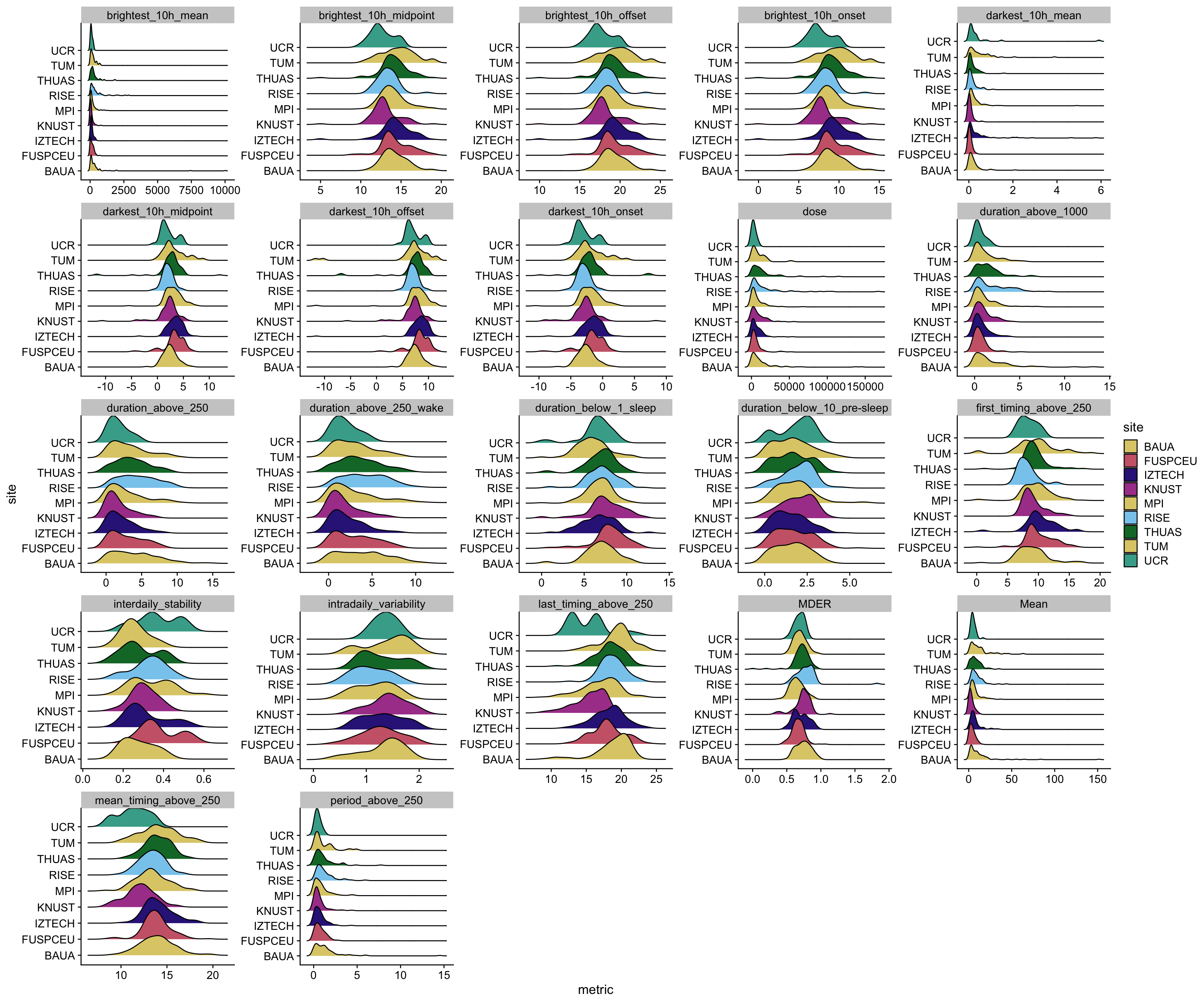
### Distributional characteristics
```{r}
#| fig-width: 18
#| fig-height: 15
#| message: false
metrics_glasses |>
  unnest(data) |>
  ggplot(aes(x=metric)) +
  geom_density_ridges(aes(y=site, fill = site))+
  facet_wrap(~ name, scales = "free") +
  scale_fill_manual(values = melidos_colors) +
  theme_cowplot()
ggsave("figures/exploration/metric_distribution_glasses.pdf", width = 18, height = 15)
```
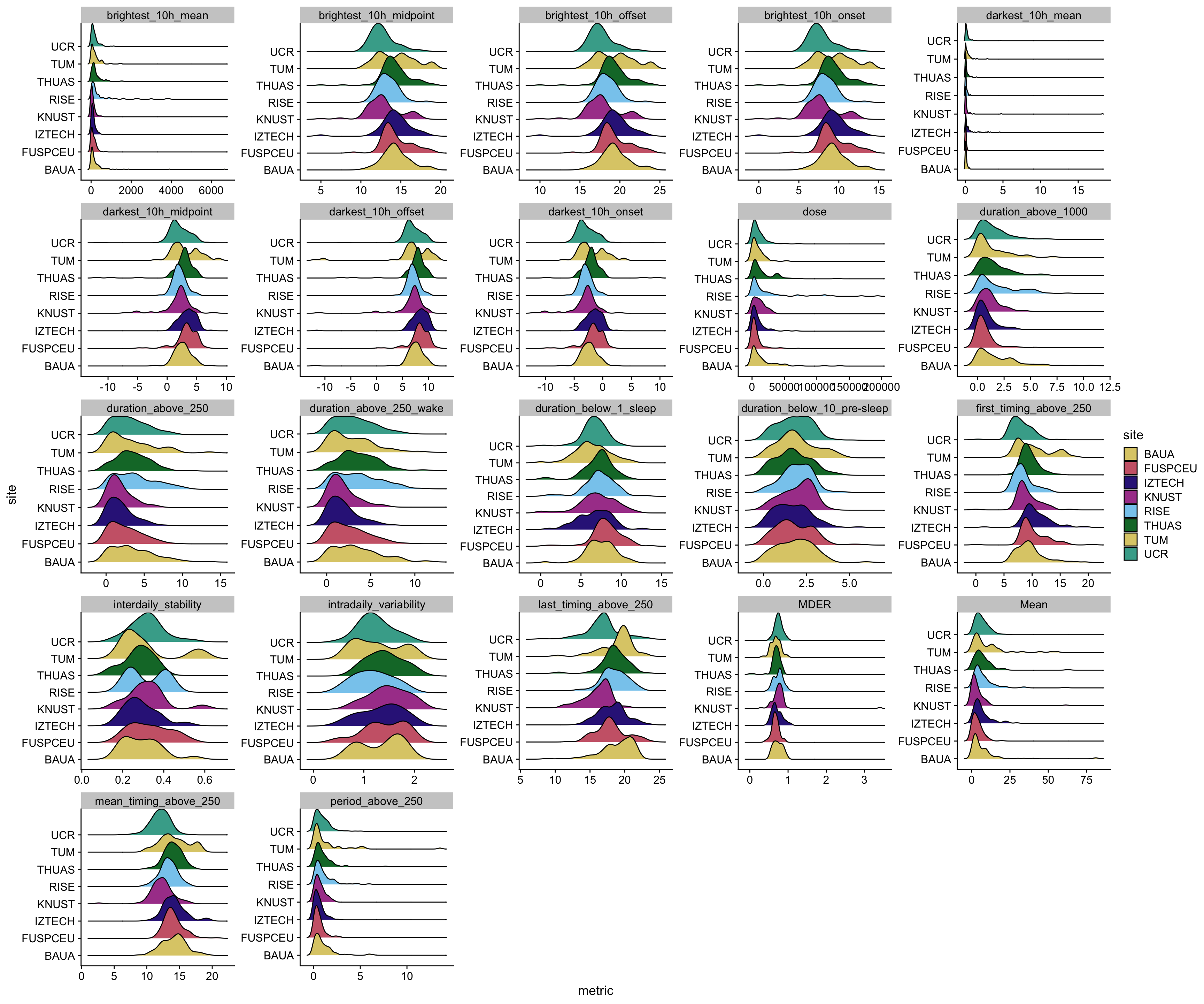
```{r}
#| fig-width: 18
#| fig-height: 15
#| message: false
metrics_chest |>
  unnest(data) |>
  ggplot(aes(x=metric)) +
  geom_density_ridges(aes(y=site, fill = site))+
  facet_wrap(~ name, scales = "free") +
  scale_fill_manual(values = melidos_colors) +
  theme_cowplot()
ggsave("figures/exploration/metric_distribution_chest.pdf", width = 18, height = 15)
```
### Export data
```{r}
save(metrics_glasses, file = "data/metrics_glasses.RData")
save(metrics_chest, file = "data/metrics_chest.RData")
```