---
title: "Research Question 2"
subtitle: "Is there a relationship between personal light exposure and participants’ behaviour and environment?"
author: "Johannes Zauner"
format:
html:
toc: true
code-tools: true
code-link: true
page-layout: full
code-fold: show
---
## Preface
This document contains the analysis for Research Question 2, as defined in the [preregistration]( https://aspredicted.org/te3zw2.pdf).
> **Research Question 2**: \
Is there a relationship between personal light exposure and participants’ behaviour and environment?
>
> *H3*: There is a significant relationship between hourly self-reported light exposure categories and hourly geometric mean of melanopic EDI.
>
> *H4*: There is a significant relationship between hourly self-reported activities and hourly geometric mean of melanopic EDI.
>
> *H5*: There is a significant relationship between LEBA-factors and pre-selected personal light exposure metrics.
>
> *H6*: There is a significant relationship between day type, daily exercise, sleep, and the hourly geometric mean of light exposure.
>
> *H7*: There is a ceiling effect of (absolute) latitude and photoperiod with level, duration, and exposure-history-based metrics
## Setup
In this section, we load in the [preprocessed](data_preparation.qmd) and [prepared](metric_preparation.qmd) data, site data, and load required packages.
```{r}
#| message: false
#| warning: false
#| code-summary: Code cell - Setup
library(tidyverse)
library(melidosData)
library(LightLogR)
library(mgcv)
library(lme4)
library(performance)
library(cowplot)
library(ggridges)
library(ggtext)
library(sjPlot)
library(broom)
library(itsadug)
library(gratia)
library(emmeans)
library(patchwork)
library(rlang)
library(broom.mixed)
library(gt)
library(performance)
library(glmmTMB)
library(gghighlight)
library(gtsummary)
source("scripts/fitting.R")
source("scripts/summaries.R")
source("scripts/RQ2_specific.R")
```
```{r}
#| message: false
#| file-name: Load data
load("data/metrics_glasses.RData")
load("data/preprocessed_glasses_2.RData")
metrics <- metrics_glasses
hourly_data <-  light_glasses_processed2
H3 <- "Hypothesis: There is a significant relationship between hourly self-reported light exposure categories and hourly geometric mean of melanopic EDI."
H4 <- "Hypothesis: There is a significant relationship between hourly self-reported activities and hourly geometric mean of melanopic EDI."
H5 <- "Hypothesis: There is a significant relationship between LEBA-factors and pre-selected personal light exposure metrics."
H6 <- "Hypothesis: There is a significant relationship between the day type, daily exercise, and sleep with the hourly geometric mean of light exposure"
H7 <- "Hypothesis: There is a ceiling effect of photoperiod with level, duration, and exposure-history-based metrics."
sig.level <- 0.05

#for chest:
# load("data/metrics_chest.RData")
# metrics <- metrics_chest
# melidos_cities <- melidos_cities[names(melidos_cities)!="MPI"]
```
## Hypothesis 3
### Details
Hypothesis 3 states:
> There is a significant relationship between hourly self-reported light exposure categories and hourly geometric mean of melanopic EDI.
*Type of model:* GLMM
*Base formula:* $\text{mel EDI} \sim \text{mH-LEA}*\text{Site} + (1|\text{Site}:\text{Participant})$
*Notes:*
- site as a random effect with random slopes for mH-LEA was unstable. Thus, site will be used as an interaction
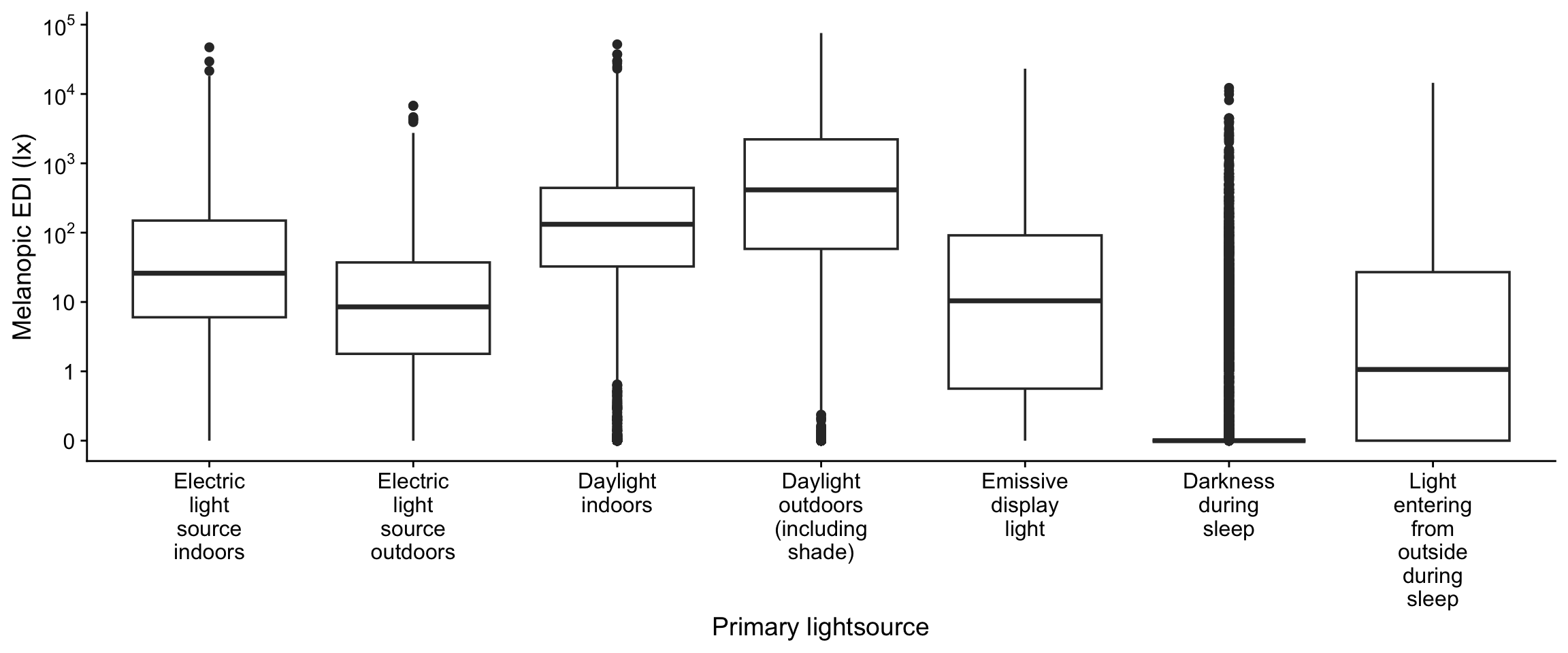
- mH-LEA data was used to collect the `primary_lightsource`, which is the variable used in the model
- The confirmatory test looks at the base model compared to the Null model for mH-LEA, the other comparisons are exploratory
- Site was sum-coded, so as to calculate an average effect of site
- Error family is Tweedie
*Specific formulas:*
- $\text{mel EDI} \sim \text{Site} + (1|\text{Site}:\text{Participant})$ (Null-model, mH-LEA)
- $\text{mel EDI} \sim \text{mH-LEA} + \text{Site} + (1|\text{Site}:\text{Participant})$ (Null-model interaction)
- $\text{mel EDI} \sim \text{mH-LEA} + (1|\text{Site}:\text{Participant})$ (Null-model, Site)
*False-discovery-rate correction:*
- non for confirmatory test (1 comparison)
- 9 for site-effects
- 4 for mH-LEA
### Preparation
```{r}
#| filename: Load hourly self-reported light exposure
mHLEA <- load_data("lightexposurediary") |> flatten_data()
mHLEA_labels <-
  mHLEA|> extract_labels() |>
  enframe() |>
  filter(str_detect(name, "act_")) |>
  mutate(name = name |> str_remove("act_"))
```
```{r}
hourly_data <-
  hourly_data |>
  aggregate_Datetime(
    "1 hour",
    type = "floor",
    numeric.handler = \(x) x |> mean(na.rm = TRUE),
    geo.MEDI = MEDI |> log_zero_inflated() |> mean(na.rm = TRUE) |> exp_zero_inflated()
  )|>
  add_Date_col(group.by = TRUE) |>
  mutate(static = all(MEDI == MEDI[1])) |>
  filter_out(static) |>
  select(-static) |>
  ungroup(Date)
```
```{r}
#| filename: Merge light data with self-reports
hourly_data <-
  hourly_data |>
  group_by(site, Id, Date) |>
  add_states(mHLEA)
```
```{r}
#| filename: Plot overview of light against self-reports
#| fig-width: 12
#| fig-height: 5

addline_format <- function(x,...){
    gsub('\\s','\n',x)
}

hourly_data |>
  filter_out(is.na(lightsource_primary)) |>
  ggplot(aes(x=lightsource_primary, y = MEDI)) +
  geom_boxplot() +
  scale_x_discrete(labels = addline_format) +
  scale_y_continuous(trans = "symlog",
                     breaks = c(0,1,10,100,1000,10000,10^5),
                     labels = expression(0,1,10,10^2,10^3,10^4,10^5)) +
  theme_cowplot() +
  labs(y = "Melanopic EDI (lx)", x = "Primary lightsource")
```
```{r}
hourly_data |>
  ungroup() |>
  count(lightsource_primary) |>
  mutate(pct = (n / sum(n))) |>
  gt() |> fmt_percent(pct, decimals = 0)
```
We will remove any subgroup that has less than 0.1 % of the total datapoints, i.e., 20 observations within a site, and then 1% less than overall, i.e., 200 observations. We will also drop "Light entering from outside during sleep", as it is very unevenly populated and dropped site levels will lead to issues later.
```{r}
hourly_data2 <-
  hourly_data |>
  group_by(site, lightsource_primary) |>
  mutate(n = n(),
         lightsource_primary = lightsource_primary |>
           replace_when((n < 20 ) ~ NA)
           ) |>
  group_by(lightsource_primary) |>
  mutate(n = n(),
         lightsource_primary = lightsource_primary |>
           replace_when((n < 200 ) ~ NA,
                        lightsource_primary == "Light entering from outside during sleep" ~ NA),
         site = factor(site)
           )
```
```{r}
library(nnet)
hourly_data3 <- hourly_data2 |> mutate(lightsource_primary = fct_drop(lightsource_primary))
model_lightsource_site <- multinom(
  lightsource_primary ~ site,
  data = hourly_data3
)
model_lightsource_site0 <- multinom(
  lightsource_primary ~ 1,
  data = hourly_data3
)
anova(model_lightsource_site, model_lightsource_site0, test = "Chisq")
prop.table(
  table(hourly_data3$site, hourly_data3$lightsource_primary),
  margin = 1)
chisq.test(table(hourly_data3$site, hourly_data3$lightsource_primary))
```
### Analysis
```{r}
#| filename: Fit the model for H3
#| fig-height: 10
#| fig-width: 8
H3_formula_1 <- geo.MEDI ~ site*lightsource_primary + (1|Id)
H3_formula_0 <- geo.MEDI ~ site + (1|Id)
H3_formula_1_ni <- geo.MEDI ~ site + lightsource_primary + (1|Id)
H3_formula_1_ns <- geo.MEDI ~ lightsource_primary + (1|Id)

#confirmatory
H3_model_1 <-
  glmmTMB(H3_formula_1,
          data = hourly_data2 |> drop_na(lightsource_primary),
          REML = FALSE,
          family = tweedie(),
          contrasts = list(site = "contr.sum")
          )
H3_model_0 <-
  glmmTMB(H3_formula_0,
          data = hourly_data2 |> drop_na(lightsource_primary),
          REML = FALSE,
          family = tweedie(),
          contrasts = list(site = "contr.sum")
          )
#exploratory:
H3_model_1_ni <-
  glmmTMB(H3_formula_1_ni,
          data = hourly_data2 |> drop_na(lightsource_primary),
          REML = FALSE,
          family = tweedie(),
          contrasts = list(site = "contr.sum")
          )
H3_model_1_ns <-
  glmmTMB(H3_formula_1_ns,
          data = hourly_data2 |> drop_na(lightsource_primary),
          REML = FALSE,
          family = tweedie(),
          )

comp_confirmatory <-
anova(H3_model_0, H3_model_1)
comp_confirmatory
comp_interaction <-
anova(H3_model_1, H3_model_1_ni)
comp_interaction
comp_site <-
anova(H3_model_1_ns, H3_model_1_ni)
comp_site
AIC(H3_model_1_ni, H3_model_1, H3_model_0, H3_model_1_ns) |>
arrange(AIC) |>
rownames_to_column("model") |> gt()
```
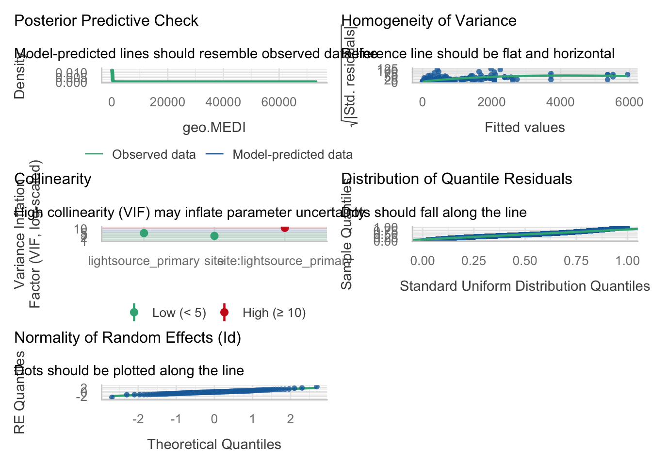
Both AIC and ∆loglik comparisons suggest that the interaction model is the most relevant one.
```{r}
check_model(H3_model_1)
```
```{r}
tab_model(H3_model_1, CSS = css_theme("cells"))
```
#### Basic table
```{r}
H3_tab_ran <-
  H3_model_1 |>
  tidy() |>
  mutate(signif = p.value <= sig.level,
         estimate = exp(estimate) |> round(2)) |>
  filter(effect == "ran_pars") |>
  select(term, estimate)

H3_tab_reference <-
  H3_model_1 |>
  emmeans(~ lightsource_primary, type = "response",
          at = list(lightsource_primary = "Electric light source indoors")) |>
  as_tibble() |>
  rename(estimate = response)
H3_tab_light <-
  H3_model_1 |>
  emmeans(~ lightsource_primary, type = "response") |>
  contrast(method = "trt.vs.ctrl") |>
  as_tibble() |>
  rename(estimate = ratio)
H3_tab_interaction <-
  H3_model_1 |>
  emmeans(~ site | lightsource_primary, type = "response") |>
  contrast() |>
  as_tibble() |>
  rename(estimate = ratio)

H3_tab_fix <-
  bind_rows(H3_tab_reference, H3_tab_light, H3_tab_interaction) |>
  mutate(signif = p.value <= sig.level) |>
  select(-c(df, asymp.LCL, asymp.UCL, null, z.ratio)) |>
  relocate(contrast, .before = 1) |>
  mutate(site = contrast |> as.character(),
         lightsource_primary =
           lightsource_primary |> as.character() |>
           replace_when(
             str_detect(contrast, "Electric light source indoors") ~ str_remove(contrast, " / Electric light source indoors")
           ),
         site = replace_when(site,
                             is.na(site) ~ "Overall",
                             str_detect(site, " effect") ~ str_remove(site, " effect"),
                             str_detect(contrast, "Electric light source indoors") ~ "Overall"),
         .before = 1

  ) |>
  select(-contrast) |>
  pivot_wider(id_cols = site, names_from = lightsource_primary, values_from = estimate:signif)
  # mutate(
         # across(3:6,
                # \(x) c(x[1], x[-1]*x[1]))
         # )
```
```{r}
H3_r2_1 <- r2_helper(H3_model_1, hourly_data2 |> drop_na(lightsource_primary), tweedie(), "geo.MEDI", "(1 | Id)")
H3_r2_0 <- r2_helper(H3_model_0, hourly_data2 |> drop_na(lightsource_primary), tweedie(), "geo.MEDI", "(1 | Id)")
H3_r2_interaction<- r2_helper(H3_model_1_ni, hourly_data2 |> drop_na(lightsource_primary), tweedie(), "geo.MEDI", "(1 | Id)")
H3_r2_site<- r2_helper(H3_model_1_ns, hourly_data2 |> drop_na(lightsource_primary), tweedie(), "geo.MEDI", "(1 | Id)")
H3_tab_r2 <-
  tribble(
    ~type, ~r2,
    "Model", H3_r2_1$R2_conditional,
    "All fixed", H3_r2_1$R2_marginal,
    "Residual", 1-H3_r2_1$R2_conditional,
    "Lightsource", H3_r2_1$R2_marginal - H3_r2_0$R2_marginal,
    "Site", H3_r2_1$R2_marginal - H3_r2_site$R2_marginal,
    "Random", H3_r2_1$R2_conditional - H3_r2_1$R2_marginal,
    "Interaction", H3_r2_1$R2_marginal - H3_r2_interaction$R2_marginal,
  ) |>
  mutate(r2= r2 |> round(2))
```
```{r}
H3_tab <-
H3_tab_fix |>
  site_conv_mutate(rev = FALSE, other.levels = "Overall") |>
  arrange(site) |>
  gt() |>
  cols_label_with(fn = \(x) str_remove(x, "estimate_") |> str_remove("lightsource_primary")) |>
  tab_spanner(
    md(
      paste0("Primary lightsource ($p = ",
             comp_confirmatory$`Pr(>Chisq)`[2] |> style_pvalue(),
             "$, $R^2=", H3_tab_r2$r2[4],
             "$)")
      ),
    columns = -site) |>
  cols_hide((contains(c("p.value", "signif", "SE_")))) |>
  sub_missing(missing_text = "") |>
  tab_style_body(
    style = cell_borders(weight = px(2)),
    rows = 1,
    columns = 2,
    fn = \(x) TRUE
  ) |>
  gt::rows_add(site = NA, .after = 1) |>
  tab_style(
    style = list(css(`padding-top` = "0px",
            `padding-bottom` = "0px"),
            cell_fill("lightgrey")
            ),
locations = cells_body(rows = 2)) |>
  fmt(starts_with("estimate"),
      fns = \(x)
      {x <- x |> gt::vec_fmt_number()
      str_c(x, "×")}
      ) |>
  fmt(columns = 2,
      rows = site == "Overall",
      fns = \(x)
      {x <- x |> gt::vec_fmt_number()
      str_c(x, "lx")}
      ) |>
  gt_multiple(
    names(H3_tab_fix) |>
      subset(str_detect(names(H3_tab_fix), "estimate_")) |>
      str_remove("estimate_"),
    bold_p.) |>
  gt_multiple(
    melidos_colors |> names(),
    style_rows
  ) |>
  tab_style(
    style = cell_text(weight = "bold"),
    locations = list(
      cells_column_labels(),
      cells_column_spanners(),
      cells_body(columns = site),
      cells_body(2,1)
    )
  ) |>
  cols_label(
    site = md(paste0("Site<br>($p = ",
             comp_site$`Pr(>Chisq)`[2] |> style_pvalue(),
             "$, $R^2=", H3_tab_r2$r2[5],
             "$)"))
    ) |>
  tab_header(
    title = "Model results for Hypothesis 3",
    subtitle = H3
  ) |>
  tab_footnote(
    "Reference value, for electric light indoors and a site average. All other values have to be multiplied by the reference value, their respective `Overall` multiplier, and optionally the site interaction to get the estimated mel EDI for a given combination.", locations = cells_body(2,1)
  ) |>
  tab_footnote(
    md(paste0("Conditional (Model) $R^2=",
              H3_tab_r2$r2[1],
              "$, Marginal (Fixed effects) $R^2=",
              H3_tab_r2$r2[2],
              "$, Random effect $R^2=",
              H3_tab_r2$r2[6],
              "$, Residual Variance $R^2=",
              H3_tab_r2$r2[3],
              "$; Random effect of participant: $×",
              H3_tab_ran$estimate[1],
              "$; Model based on ",
              hourly_data2 |> drop_na(geo.MEDI, lightsource_primary) |> nrow() |> vec_fmt_integer(sep_mark = "'"),
              " participant-hours."
              ))
  ) |>
  tab_footnote(
    md(paste0("Interaction effect of primary lightsource with site is significant ($p=",
              comp_interaction$`Pr(>Chisq)`[2] |> style_pvalue(),
              "$, $R^2 = ",
              H3_tab_r2$r2[7],
              "$)"))
  ) |>
  tab_footnote(
    md("Values shown in **bold** are significant at $p<0.05$. False-discovery-rate adjustment for n=4 in primary lightsource and n=9 in site")
  ) |>
  cols_width(everything() ~ px(150))
```
```{r}
H3_tab
gtsave(H3_tab, "tables/H3.png")
gtsave(H3_tab, "tables/H3.docx")
```
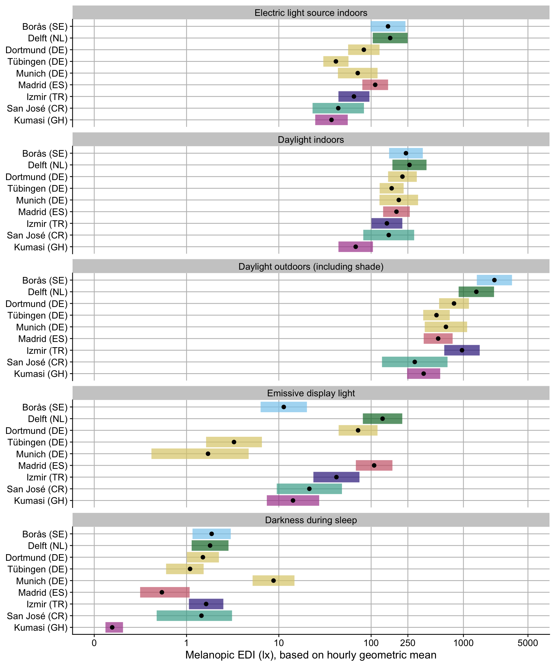
#### Visualization
```{r}
#| filename: visualize H3 result
#| fig-width: 10
#| fig-height: 12
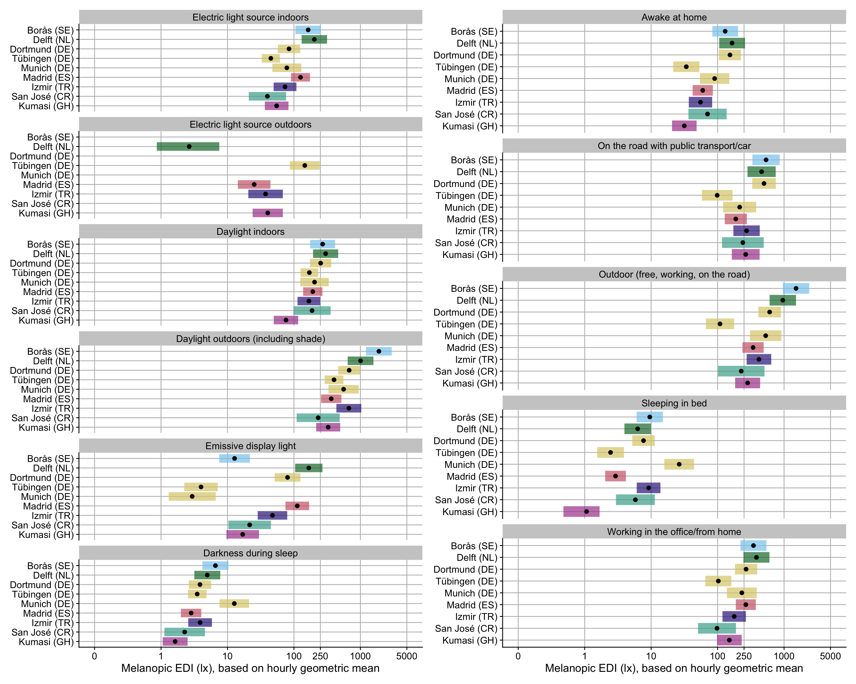
H3_plot <-
H3_model_1 |>
emmeans(~ site | lightsource_primary, type = "response") |>
plot()
H3_plot <-
H3_plot$data |>
as.tibble() |>
site_conv_mutate(site = pri.fac) |>
ggplot(
aes(x = the.emmean, y = pri.fac)
) +
geom_crossbar(aes(xmin = lcl, xmax = ucl, fill = pri.fac), col = NA, alpha = 0.7) +
geom_point() +
theme_cowplot() +
theme(panel.grid.major = element_line(color = "grey")) +
scale_fill_manual(values = melidos_colors) +
facet_wrap(~lightsource_primary, ncol = 1) +
scale_x_continuous(trans = "symlog", breaks = c(0, 10^(0:5), 250, 5000)) +
coord_cartesian(xlim = c(0, 5000)) +
labs(y = NULL, x = "Melanopic EDI (lx), based on hourly geometric mean") +
guides(fill = "none")
H3_plot
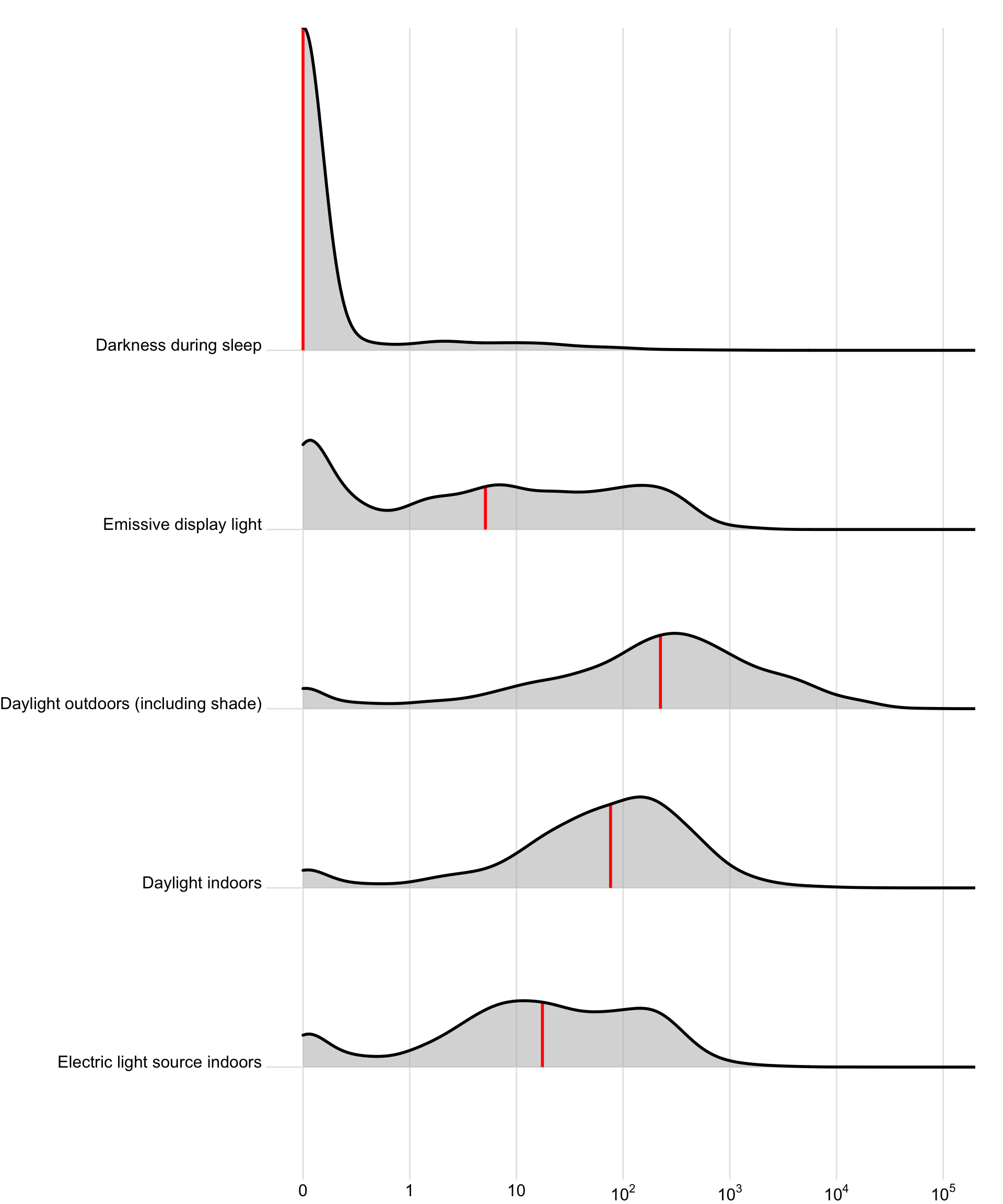
hourly_data2 |>
filter_out(is.na(lightsource_primary)) |>
site_conv_mutate(rev = FALSE) |>
ggplot(aes(x=geo.MEDI)) +
geom_density_ridges(aes(y=lightsource_primary),
linewidth = 1, colour = NA,
alpha = 0.5,
from = 0,
) +
geom_density_ridges(aes(y=lightsource_primary), fill = NA,
alpha = 1, linewidth = 1,
quantile_lines = TRUE, quantiles = 2, vline_color = "red",
linetype = 1,
from = 0,
) +
# scale_fill_manual(values = melidos_colors) +
scale_alpha_continuous(range = c(0, 1)) +
scale_x_continuous(trans = "symlog", breaks = c(0, 10^(0:5)),
labels = expression(0, 1, 10, 10^2, 10^3, 10^4, 10^5)) +
# scale_color_manual(values = melidos_colors) +
guides(fill = "none", color = "none") +
labs(y = NULL, x = NULL) +
theme_ridges() +
coord_cartesian(xlim = c(0, 10^5)) +
theme_sub_plot(margin = margin(r = 20, t = 20)) +
theme_sub_axis_left(text = element_text(vjust = 0))
```
### Interpretation
- Overall, an average mel EDI of 74.1 lx (based on geometric mean) is reached with `electric light indoors`. This value somewhat varies between sites, with Sweden, The Netherlands, and Madrid achieving substantially higher values (factor 2.06, 2.17, and 1.49, respectively). They nevertheless do not reach recommended values of 250lx during the day. Tübingen, Germany, and Ghana reach significantly lower levels (factor 0.56 and 0.5, respectively).
- When the primary lightsource is `Daylight indoors`, about 2.34 times as much mel EDI can be achieved on average (173.4 lx). The only significant deviation is Ghana, which scores 61% less than the other sites (factor 0.39).
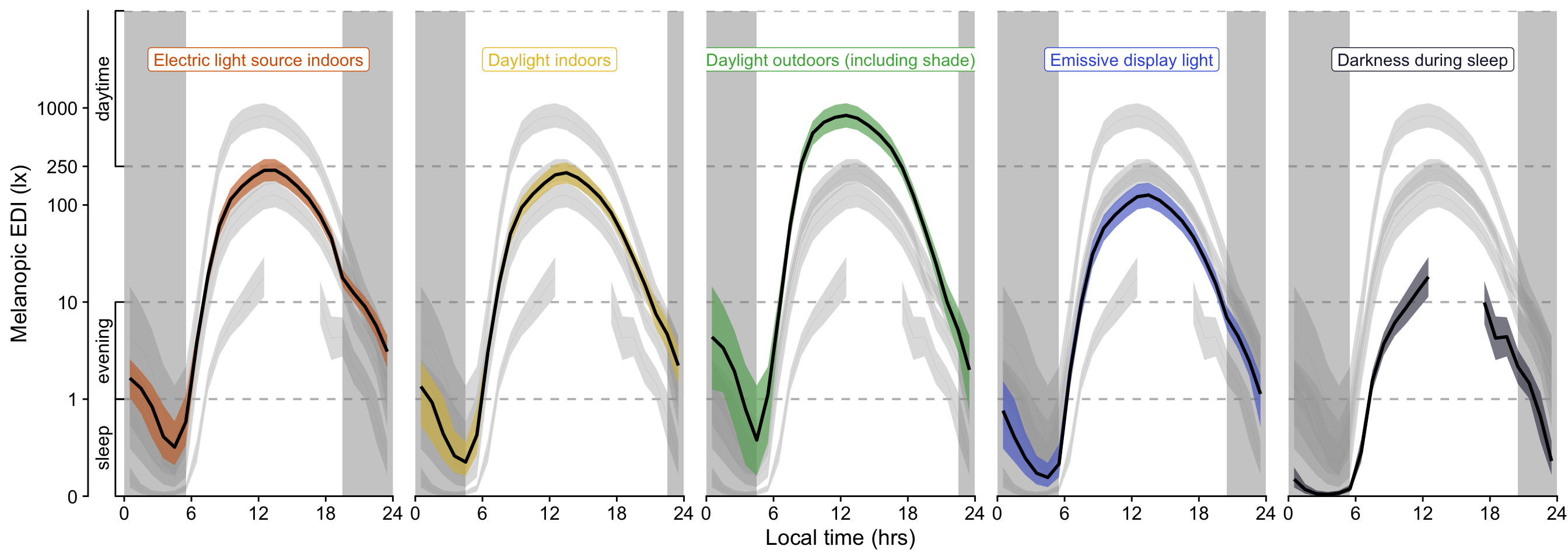
- When people are receiving `Daylight outdoors (including shade)`, they achieve about 9.81 times more light compared to `indoor electric light` (727 lx). Sweden and the Netherlands achieve still higher values (times 2.98 and 1.9, respectively), while Ghana has only about half (0.51)
- `Emissive display light` as the primary lightsource leads to values of melanopic EDI of 29% of `indoor electric light` (21.5 lx). There is very high variance between the different sites, with factor ranging between 8% (Munich, Germany) to 623% (The Netherlands).
- `Darkness during sleep` translates to about 2% of light levels compared to `indoor electric light` (~1.5 lx). Values are similar across sites, with three notable exceptions: Munich, Germany has over 6 times the level compared to other sites (6.61), while Spain and Ghana have considerably lower values (0.55 and 0.15, respectively).
- Overall, the effect of self-reported primary lightsource is astounding - 71% of variance can be explained simply through those categories. While site and interindividual differences are significant, they contribute considerably less (5% and 7%, respectively).
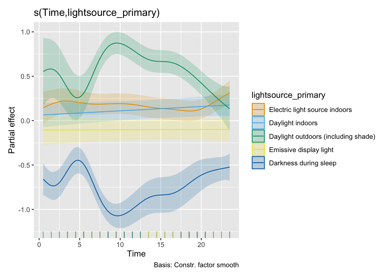
### Exploration: GAM of lightsource x time
In this exploratory analysis, we study the nonlinear effect of time on the type of primary lightsource, based on the final model from RQ1:
```{r}
#| filename: Prepare GAM data
GAM_data <-
  hourly_data2 |>
  add_Time_col() |>
  drop_na(lightsource_primary) |>
  ungroup() |>
  mutate(Time = as.numeric(Time)/3600 + 0.5,
         across(c(site, Id, sleep, State.Brown, wear, photoperiod.state,
                  lightsource_primary, Date),
                factor),
         Id_date = interaction(Id, Date),
         lzMEDI = log_zero_inflated(MEDI),
         photoperiod = (dusk - dawn) |> as.numeric()
  ) |>
  group_by(Id) |>
  mutate(AR.start = ifelse(row_number() == 1, TRUE, FALSE))

H3_form_gam <- lzMEDI ~ s(Time, k = 12) + s(Time, lightsource_primary, bs = "sz", k = 12) + s(Time, site, bs = "sz", k = 12) + s(Time, photoperiod.state, bs = "sz", k=12) + s(Time, Id, bs = "fs") + s(Id_date, bs = "re")
H2_form_gam <- lzMEDI ~ s(Time, k = 12) + s(Time, site, bs = "sz", k = 12) + s(Time, photoperiod.state, bs = "sz", k=12) + s(Time, Id, bs = "fs") + s(Id_date, bs = "re")
```
```{r}
#| filename: Main model
H3_model_gam <-
bam(H3_form_gam,
data = GAM_data,
discrete = TRUE,
method = "fREML",
nthreads = 10
)
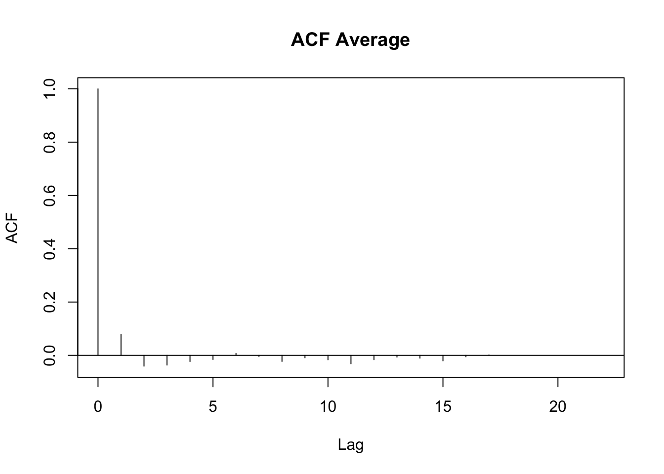
r1 <- start_value_rho(H3_model_gam,
plot=TRUE)
H3_model_gam <-
bam(H3_form_gam,
data = GAM_data,
discrete = TRUE,
method = "fREML",
nthreads = 10,
rho = r1,
AR.start = AR.start
)
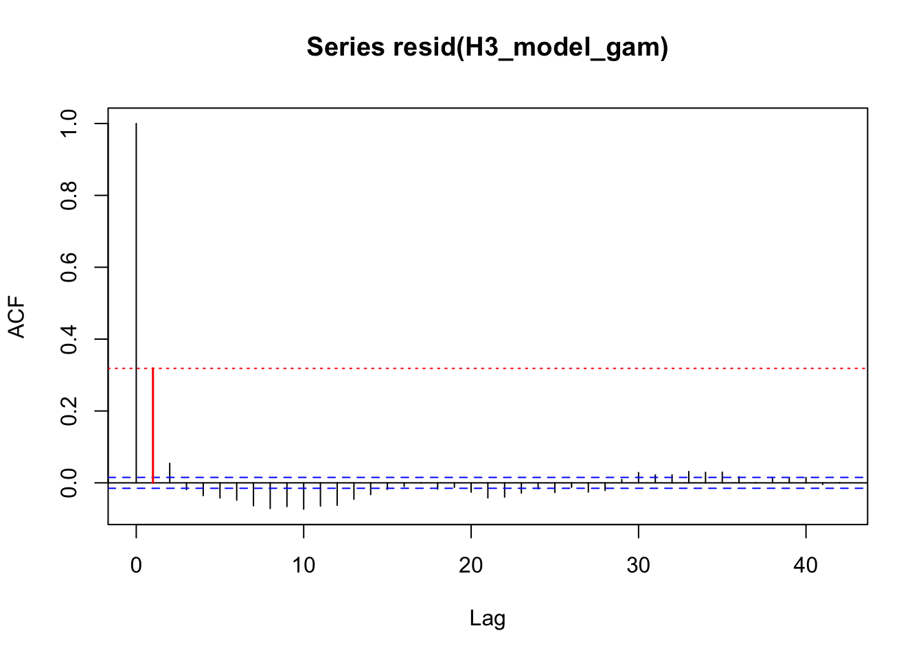
acf_resid(H3_model_gam, split_pred = "AR.start")
H3_summary_gam <- summary(H3_model_gam)
H3_summary_gam
H3_model_gam |> glance()
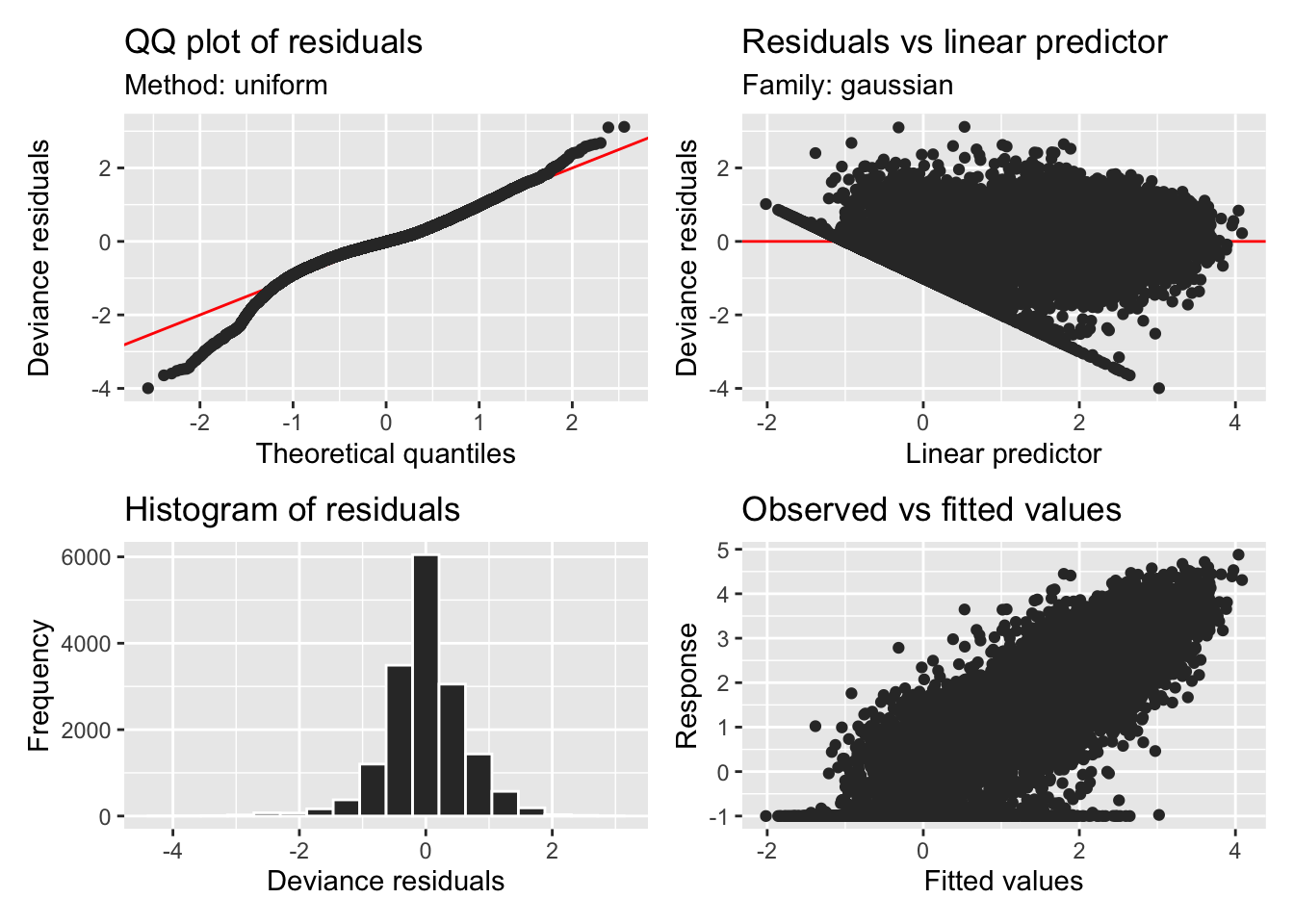
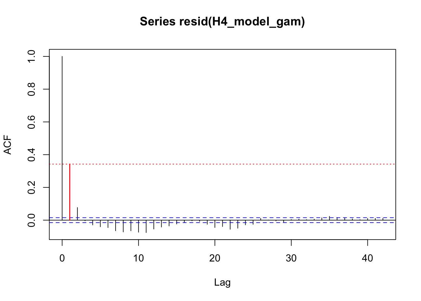
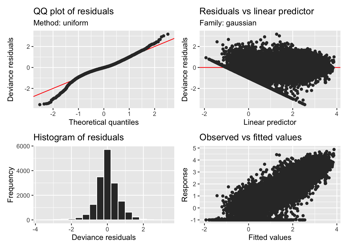
H3_model_gam |> appraise()
```
```{r}
#| filename: Variance explained
Xp <- predict(H3_model_gam, type = "terms")
variance <- apply(Xp, 2, var)
cor(Xp)
H3_R2 <- (variance/sum(variance)) |> enframe(value = "R2", name = "parameter")
H3_R2
```
```{r}
#| filename: Null model
H2_model_gam <-
  bam(H2_form_gam,
      data = GAM_data,
      discrete = TRUE,
      method = "fREML",
      nthreads = 10
      )

r1 <- start_value_rho(H2_model_gam,
                      plot=TRUE)
H2_model_gam <-
bam(H2_form_gam,
data = GAM_data,
discrete = TRUE,
method = "fREML",
nthreads = 10,
rho = r1,
AR.start = AR.start
)
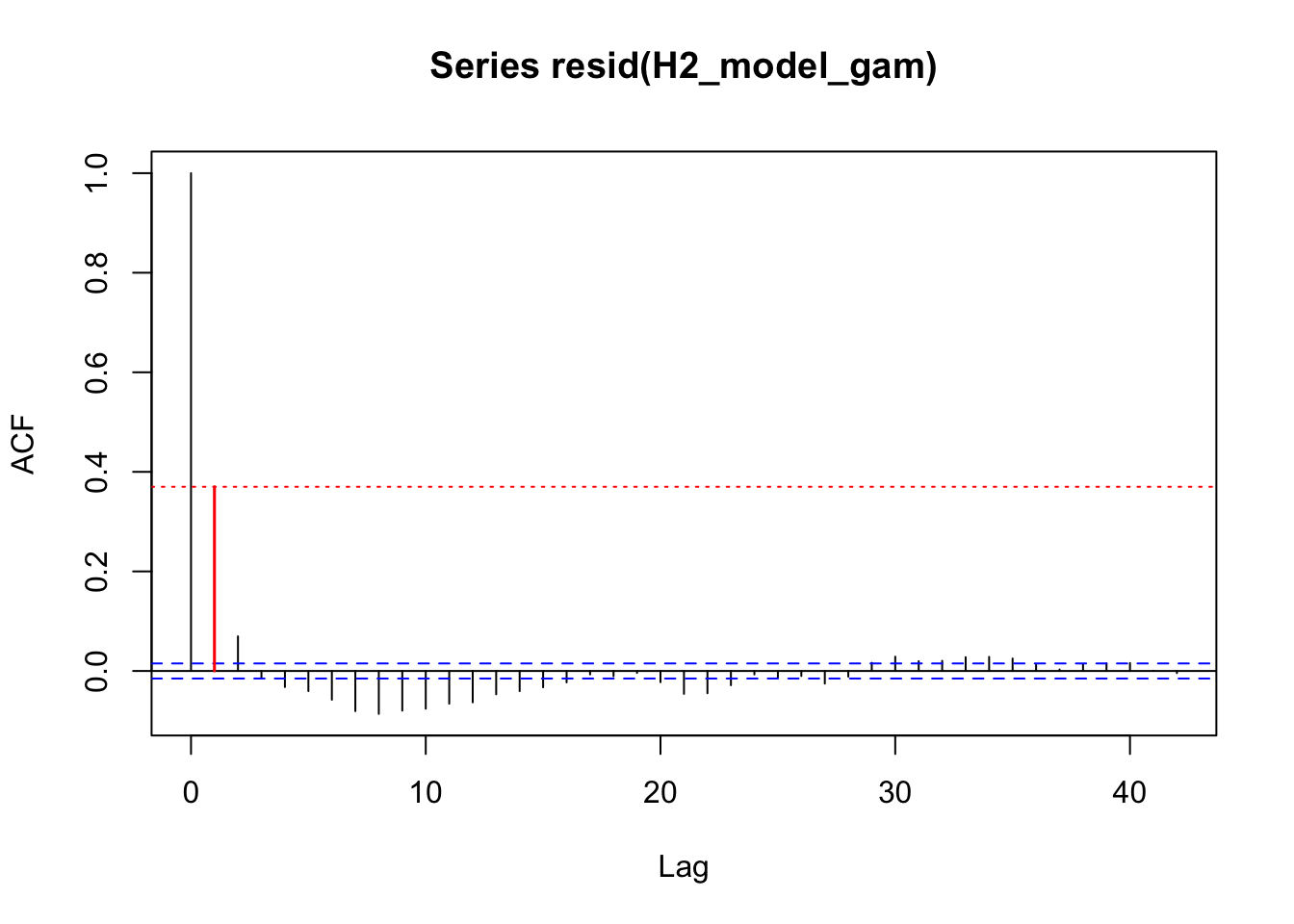
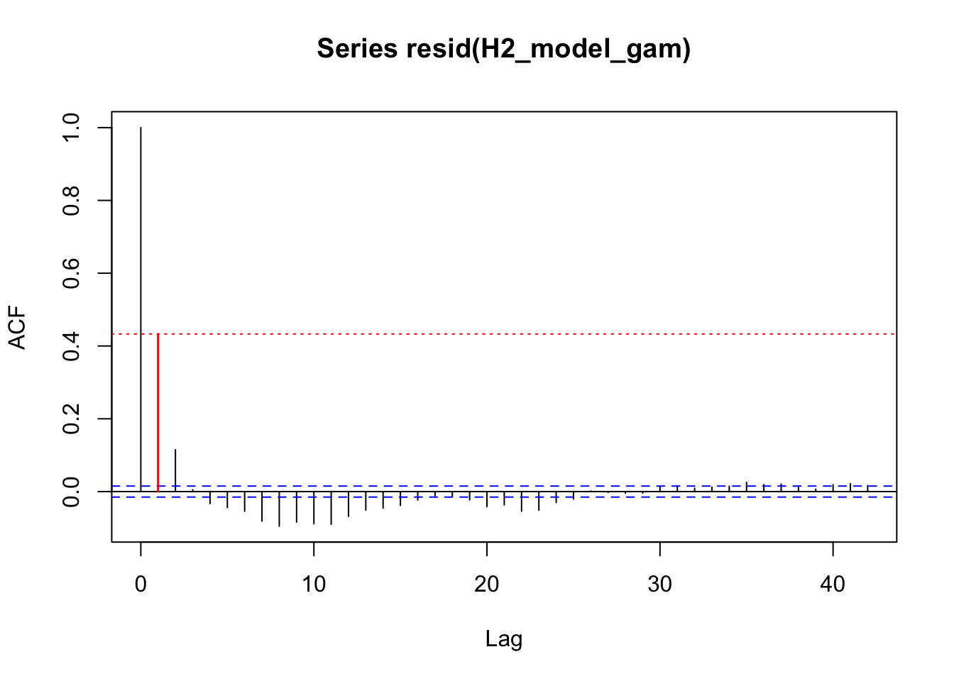
acf_resid(H2_model_gam, split_pred = "AR.start")
```
```{r}
AIC(H3_model_gam, H2_model_gam)
```
```{r}
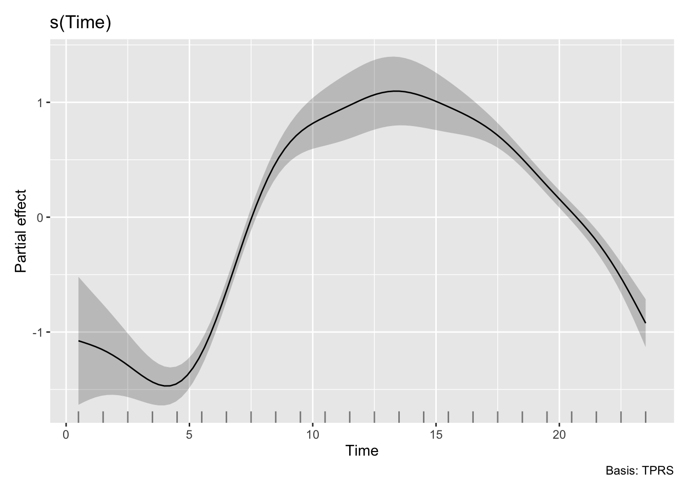
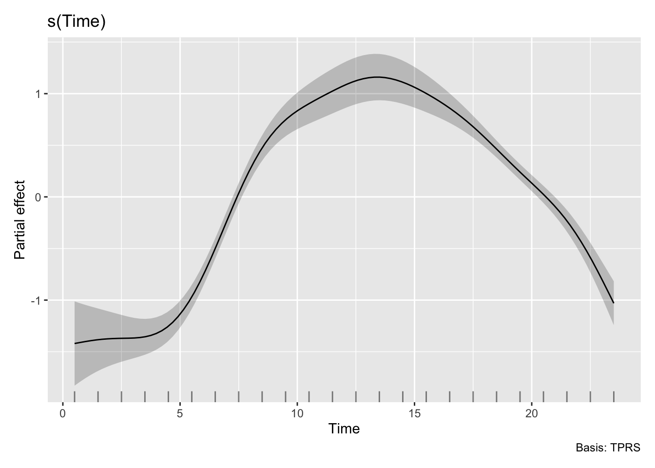
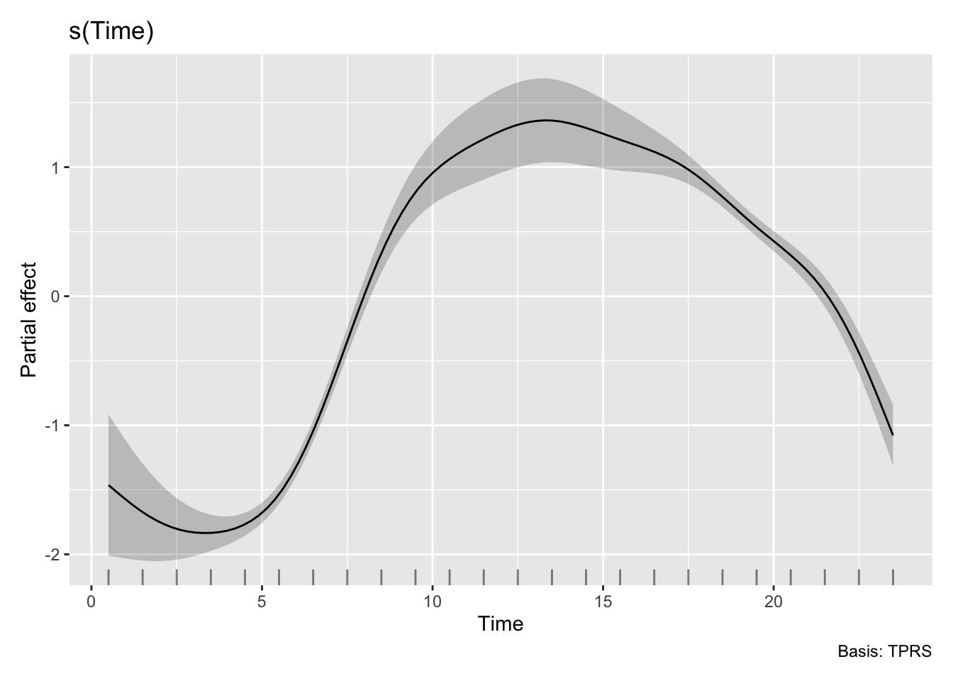
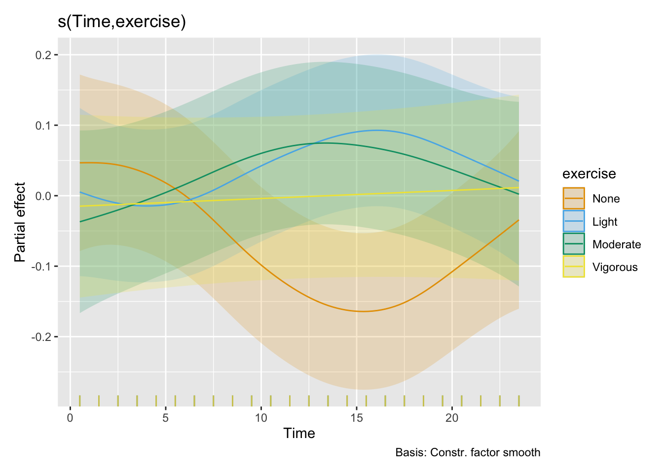
H3_model_gam |> draw(select = "s(Time,lightsource_primary)")
H3_model_gam |> draw(select = "s(Time)")
```
####Visualization
```{r}
#| filename: prepare lightsource model H3 plot
H3_ls_data <-
H3_model_gam |>
  conditional_values(
    condition = list(Time = seq(0.5, 23.5, by = 1), "lightsource_primary", "photoperiod.state"),
    exclude = c("s(Time,Id)", "s(Id_date)", "s(Time,site)")
    ) |>
  mutate(across(c(.fitted, .lower_ci, .upper_ci),
                exp_zero_inflated)
  )

H3_ls_data <-
GAM_data |>
  Datetime2Time() |>
  group_by(lightsource_primary, Time) |>
  summarize(
    .groups = "drop_last",
    dawn = dawn |> as.numeric() |> mean(na.rm = TRUE)/3600,
    dusk = dusk |> as.numeric() |> mean(na.rm = TRUE)/3600,
    n = n()
  ) |>
  mutate(
    photoperiod.state = ifelse(between(Time, dawn, dusk), "day", "night")
  ) |>
  select(-c(dawn, dusk)) |>
  left_join(H3_ls_data, by = c("lightsource_primary", "Time", "photoperiod.state"))

H3_ls_data_phot <-
H3_ls_data |>
  number_states(photoperiod.state) |>
  filter(photoperiod.state == "night") |>
  group_by(lightsource_primary, photoperiod.state.count) |>
  summarize(xmin = min(Time),
            xmax = max(Time),
            .groups = "drop_last") |>
  mutate(across(c(xmin, xmax), \(x) replace_values(x,
                                                   0.5 ~ 0,
                                                   23.5 ~ 24)))
```
```{r}
#| filename: Visualize lightsource model H3
#| fig-height: 5
#| fig-width: 14
source("scripts/Brown_bracket.R")
ls_colors <-
c(
`Darkness during sleep` = "#1B1F3B", # deep navy
`Daylight indoors` = "#E6C229", # warm yellow
`Daylight outdoors (including shade)` = "#4DAF4A", # medium leaf green
`Electric light source indoors` = "#D55E00", # amber/orange
`Emissive display light` = "#3B5BDB" # medium purple
)
H3_pred <-
H3_ls_data |>
ggplot(aes()) +
map(c(1,10,250, 10^4),
\(x) geom_hline(aes(yintercept = x),
col = "grey", linetype = "dashed")
) +
geom_rect(data = H3_ls_data_phot ,
aes(xmin = xmin, ymin = -Inf, ymax = Inf, xmax = xmax),
alpha = 0.25, inherit.aes = FALSE) +
geom_ribbon(aes(x = Time, ymin = .lower_ci,
ymax = .upper_ci, fill = lightsource_primary), alpha = 0.5) +
geom_line(aes(x = Time, y = .fitted,
col = lightsource_primary), linewidth = 0.1) +
geom_line(aes(x = Time, y = .fitted), linewidth = 1) +
scale_fill_manual(values = ls_colors) +
scale_color_manual(values = ls_colors) +
theme_cowplot() +
scale_y_continuous(trans = "symlog", breaks = c(0,1,10,100,250, 1000)) +
scale_x_continuous(breaks = seq(0, 24, by = 6)) +
coord_cartesian(xlim = c(0,24), ylim = c(0,10^4), expand = FALSE) +
labs(y = "Melanopic EDI (lx)", x = "Local time (hrs)", fill = "Primary lightsource", col = "Primary lightsource") +
facet_wrap(~lightsource_primary, nrow = 1) +
guides( y = guide_axis_stack(Brown_bracket, "axis")) +
gghighlight(
label_key = lightsource_primary,
label_params = list(x = 12, y = 4.5, force = 0, hjust = 0.5)
) +
theme_sub_strip(background = element_blank(),
text = element_blank()) +
theme(panel.spacing = unit(1, "lines"),
plot.caption = element_textbox_simple())
# labs(caption = Brown_caption)
H3_pred
```
```{r}
#| filename: Visualize model terms
Term_data <-
H3_ls_data |> select(Time, lightsource_primary) |>
left_join(
H3_model_gam |>
smooth_estimates(select = "s(Time,lightsource_primary)", n=24),
by = c("Time", "lightsource_primary")
) |>
ungroup() |>
complete(Time, lightsource_primary) |>
mutate(.lower_ci = .estimate -1.96*.se,
.upper_ci = .estimate +1.96*.se,
.fitted = .estimate,
signif = .lower_ci > 0 | .upper_ci < 0,
signif_id = consecutive_id(signif),
.by = lightsource_primary)
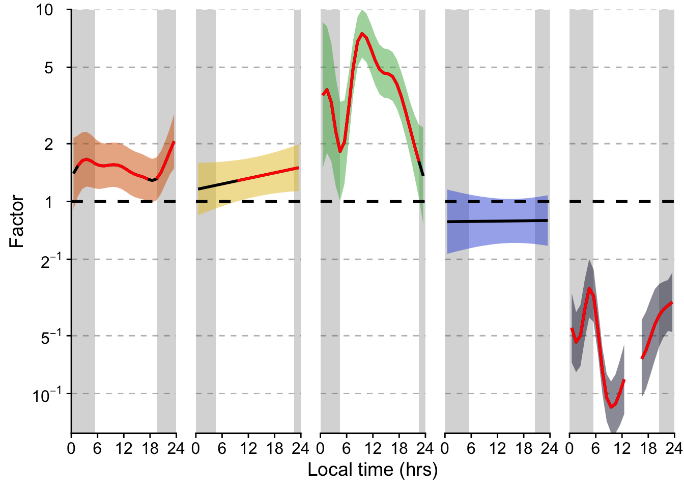
P_terms <-
Term_data |>
ggplot(aes()) +
map(c(log10(c(0.1, 0.2, 0.5, 2, 5, 10))),
\(x) geom_hline(yintercept = x, linewidth = 0.5, col = "grey", linetype = 2)) +
geom_rect(data = H3_ls_data_phot ,
aes(xmin = xmin, ymin = -Inf, ymax = Inf, xmax = xmax),
alpha = 0.25, inherit.aes = FALSE) +
geom_ribbon(aes(x = Time, ymin = .lower_ci,
ymax = .upper_ci, fill = lightsource_primary),
alpha = 0.5) +
geom_hline(yintercept = 0, linewidth = 1, linetype = 2) +
geom_line(aes(x = Time, y = .fitted),
linewidth = 1) +
geom_line(data = \(x) filter(x, signif),
aes(x = Time, y = .fitted, group = signif_id),
col = "red", linewidth = 1) +
scale_fill_manual(values = ls_colors) +
# scale_color_manual(values = c(melidos_colors)) +
theme_cowplot() +
scale_y_continuous(labels = expression(10^-1, 5^-1, 2^-1, "1 ", "2 ", "5 ", "10 "),
breaks = log10(c(0.1, 0.2, 0.5, 1, 2, 5, 10)))+
scale_x_continuous(breaks = seq(0, 24, by = 6)) +
coord_cartesian(xlim = c(0,24), expand = FALSE) +
guides(fill = "none") +
labs(y = "Factor", x = "Local time (hrs)", fill = "Primary lightsource") +
facet_wrap(~lightsource_primary, nrow = 1) +
theme_sub_strip(background = element_blank(),
text = element_blank()) +
theme(panel.spacing = unit(1, "lines"),
plot.caption = element_textbox_simple())
P_terms
```
```{r}
n_plot_H3 <-
H3_ls_data |>
  ungroup() |>
  ggplot(aes(x=Time)) +
  geom_col(aes(y=n, fill = lightsource_primary)) +
  facet_wrap(~lightsource_primary, nrow = 1) +
  theme_cowplot() +
  scale_fill_manual(values = ls_colors) +
  theme_sub_strip(background = element_blank(),
                  text = element_blank()) +
  theme(panel.spacing = unit(1, "lines"),
        plot.caption = element_textbox_simple()) +
  guides(fill = "none") +
  # scale_y_continuous(trans = "symlog", breaks = c(0, 1, 10, 100, 500)) +
  scale_x_continuous(breaks = seq(0, 24, by = 6))
```
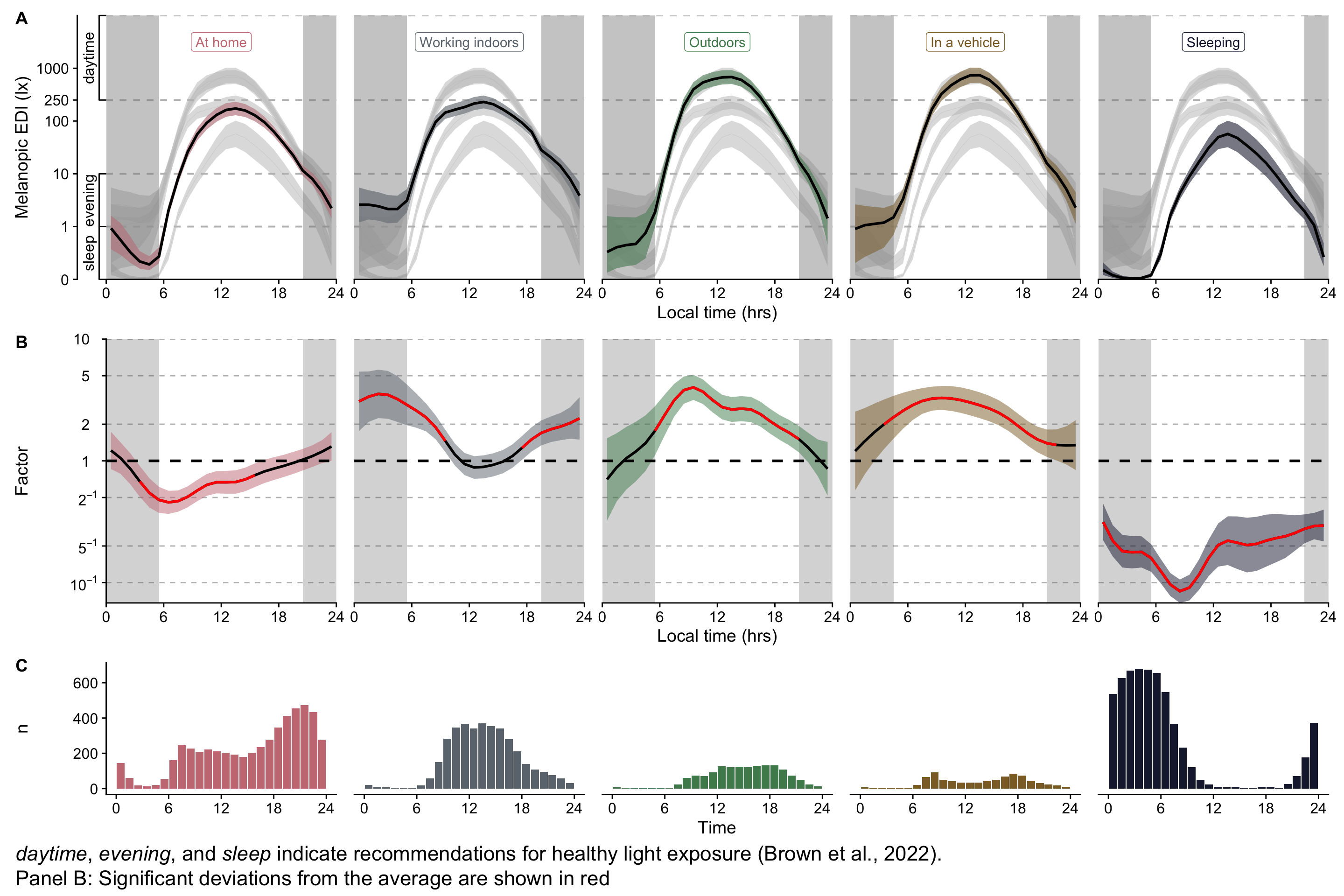
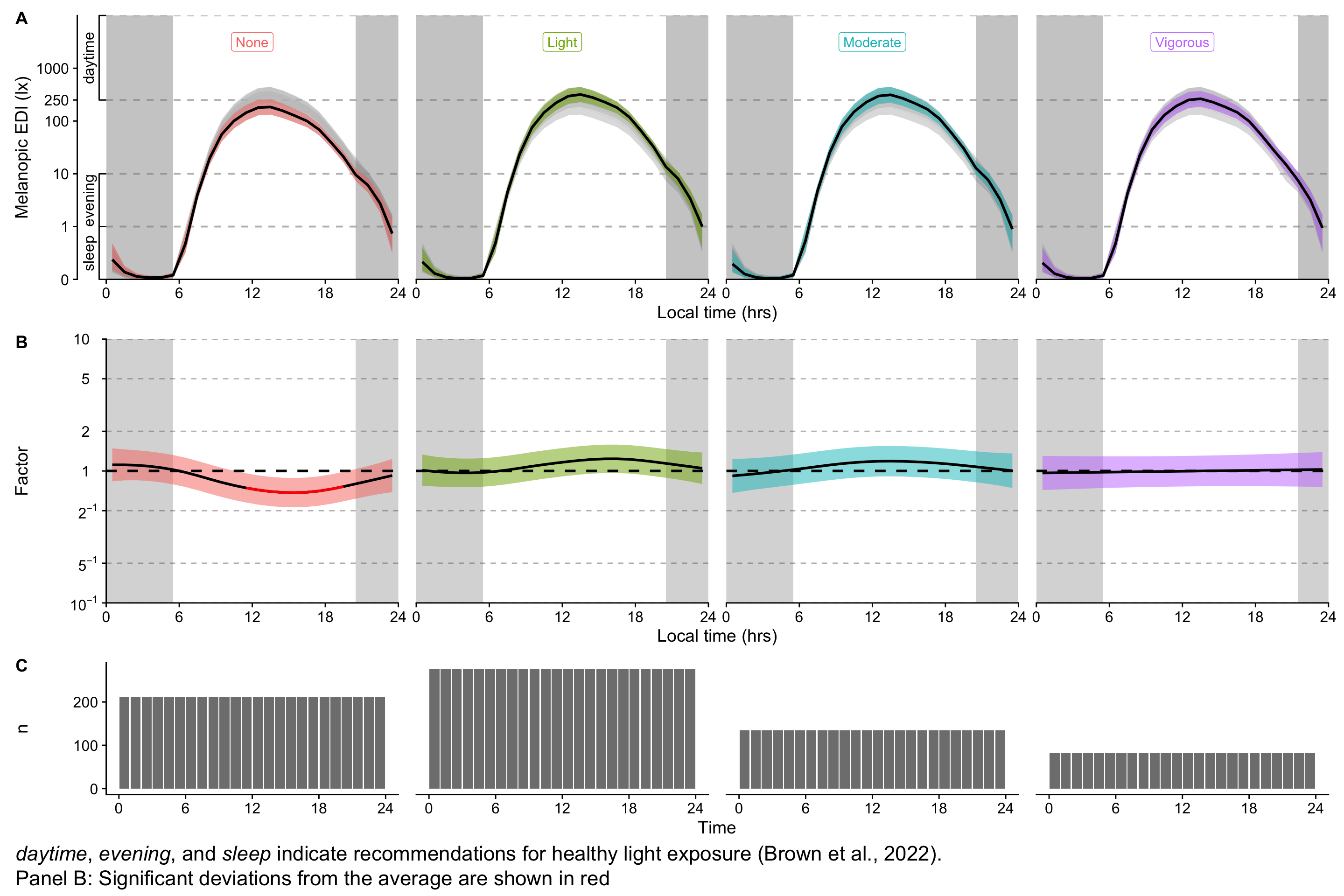
```{r}
#| fig-height: 10
#| fig-width: 15
#| filename: Combination of partial plots H3

(H3_pred / P_terms / n_plot_H3) + plot_layout(heights = c(2,2,1)) +
  plot_annotation(tag_levels = "A",
                  caption = paste(Brown_caption,
                                  "Panel B: Significant deviations from the average are shown in red", sep = "<br>"),
                  theme =
                    theme(plot.caption = element_textbox_simple(size = rel(1.5))
                          )
                  )
ggsave("figures/Fig9.pdf", height = 10, width = 15)
ggsave("figures/Fig9.png", height = 10, width = 15)
```
## Hypothesis 4
### Details
Hypothesis 4 states:
> There is a significant relationship between hourly self-reported activities and hourly geometric mean of melanopic EDI.
*Type of model:* GLMM
*Base formula:* $\text{mel EDI} \sim \text{activity}*\text{Site} + (1|\text{Site}:\text{Participant})$
*Notes:*
- site as a random effect with random slopes for activity was unstable. Thus, site will be used as an interaction
- data was used to collect various, which is the variable used in the model
- The confirmatory test looks at the base model compared to the Null model for mH-LEA, the other comparisons are exploratory
- Site was sum-coded, so as to calculate an average effect of site
- Error family is Tweedie
- We will drop the level "other" and combine outdoors levels
*Specific formulas:*
- $\text{mel EDI} \sim \text{Site} + (1|\text{Site}:\text{Participant})$ (Null-model, mH-LEA)
- $\text{mel EDI} \sim \text{mH-LEA} + \text{Site} + (1|\text{Site}:\text{Participant})$ (Null-model interaction)
- $\text{mel EDI} \sim \text{mH-LEA} + (1|\text{Site}:\text{Participant})$ (Null-model, Site)
*False-discovery-rate correction:*
- non for confirmatory test (1 comparison)
- 9 for site-effects
- 4 for activity
### Preparation
```{r}
#| filename: Prepare activity data
activity_data <-
hourly_data2 |>
  ungroup() |>
  select(site, Id, geo.MEDI, starts_with("act_"), Datetime, lightsource_primary) |>
  pivot_longer(cols = starts_with("act_"), names_to = "activity", names_prefix = "act_", values_to = "value") |>
  filter(value, !is.na(geo.MEDI)) |>
  distinct(.keep_all = TRUE, site, Id, Datetime, activity) |>
  select(-value)
```
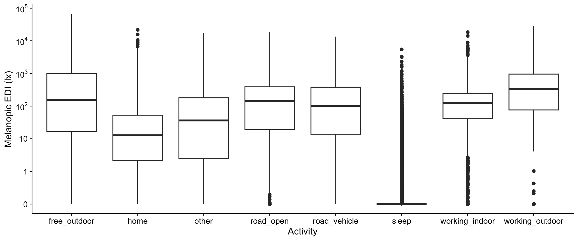
```{r}
#| filename: Plot overview of light against self-reported activity
#| fig-width: 12
#| fig-height: 5
activity_data |>
  ggplot(aes(x=activity, y = geo.MEDI)) +
  geom_boxplot() +
  scale_x_discrete(labels = addline_format) +
  scale_y_continuous(trans = "symlog",
                     breaks = c(0,1,10,100,1000,10000,10^5),
                     labels = expression(0,1,10,10^2,10^3,10^4,10^5)) +
  theme_cowplot() +
  labs(y = "Melanopic EDI (lx)", x = "Activity")
```
```{r}
activity_data |> count(activity)
```
We will drop the other group, and we will combine `working_outdoor` with `free_outdoor` and `road_open`, as they are small or non-existant in in some sites.
```{r}
activity_data <-
  activity_data |>
  mutate(activity =
           fct(activity) |>
           fct_collapse(outdoor = c("free_outdoor", "working_outdoor", "road_open")) |>
           fct_recode(NULL = "other") |>
           fct_relevel("home")
         )
```
```{r}
activity_data |> count(activity, sort = TRUE) |> mutate(pct = n / sum(n)) |> gt() |> fmt_percent(pct, decimals = 0)
activity_data <-
  activity_data |>
  drop_na(activity)
```
```{r}
library(nnet)
activity_data2 <- activity_data |> mutate(activity = fct_drop(lightsource_primary))
model_activity_site <- multinom(
  activity ~ site,
  data = activity_data2
)
model_activity_site0 <- multinom(
  activity ~ 1,
  data = activity_data2
)
anova(model_activity_site, model_activity_site0, test = "Chisq")
prop.table(
  table(activity_data2$site, activity_data2$activity),
  margin = 1)
chisq.test(table(activity_data2$site, activity_data2$activity))
```
### Analysis
```{r}
#| filename: Fit the model for H4
#| fig-height: 10
#| fig-width: 8
H4_formula_1 <- geo.MEDI ~ site*activity + (1|Id)
H4_formula_0 <- geo.MEDI ~ site + (1|Id)
H4_formula_1_ni <- geo.MEDI ~ site + activity + (1|Id)
H4_formula_1_ns <- geo.MEDI ~ activity + (1|Id)

#confirmatory
H4_model_1 <-
  glmmTMB(H4_formula_1,
          data = activity_data,
          REML = FALSE,
          family = tweedie(),
          contrasts = list(site = "contr.sum")
          )
H4_model_0 <-
  glmmTMB(H4_formula_0,
          data = activity_data,
          REML = FALSE,
          family = tweedie(),
          contrasts = list(site = "contr.sum")
          )
#exploratory:
H4_model_1_ni <-
  glmmTMB(H4_formula_1_ni,
          data = activity_data,
          REML = FALSE,
          family = tweedie(),
          contrasts = list(site = "contr.sum")
          )
H4_model_1_ns <-
  glmmTMB(H4_formula_1_ns,
          data = activity_data,
          REML = FALSE,
          family = tweedie(),
          )

comp_confirmatory <-
anova(H4_model_0, H4_model_1)
comp_confirmatory
comp_interaction <-
anova(H4_model_1, H4_model_1_ni)
comp_interaction
comp_site <-
anova(H4_model_1_ns, H4_model_1_ni)
comp_site
AIC(H4_model_1_ni, H4_model_1, H4_model_0, H4_model_1_ns) |>
arrange(AIC) |>
rownames_to_column("model") |> gt()
```
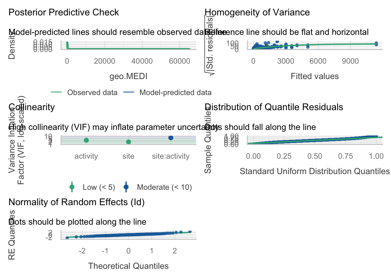
Both AIC and ∆loglik comparisons suggest that the interaction model is the most relevant one.
```{r}
check_model(H4_model_1)
```
```{r}
tab_model(H4_model_1, CSS = css_theme("cells"))
```
#### Basic table
```{r}
H4_tab_ran <-
  H4_model_1 |>
  tidy() |>
  mutate(signif = p.value <= sig.level,
         estimate = exp(estimate) |> round(2)) |>
  filter(effect == "ran_pars") |>
  select(term, estimate)

H4_tab_reference <-
  H4_model_1 |>
  emmeans(~ activity, type = "response",
          at = list(activity = "home")) |>
  as.tibble() |>
  rename(estimate = response)
H4_tab_act <-
  H4_model_1 |>
  emmeans(~ activity, type = "response") |>
  contrast(method = "trt.vs.ctrl") |>
  as.tibble() |>
  rename(estimate = ratio)
H4_tab_interaction <-
  H4_model_1 |>
  emmeans(~ site | activity, type = "response") |>
  contrast() |>
  as.tibble() |>
  rename(estimate = ratio)

H4_tab_fix <-
  bind_rows(H4_tab_reference, H4_tab_act, H4_tab_interaction) |>
  mutate(signif = p.value <= sig.level) |>
  select(-c(df, asymp.LCL, asymp.UCL, null, z.ratio)) |>
  relocate(contrast, .before = 1) |>
  mutate(site = contrast |> as.character(),
         activity =
           activity |> as.character() |>
           replace_when(
             str_detect(contrast, "home") ~ str_remove(contrast, " / home")
           ),
         site = replace_when(site,
                             is.na(site) ~ "Overall",
                             str_detect(site, " effect") ~ str_remove(site, " effect"),
                             str_detect(contrast, "home") ~ "Overall"),
         .before = 1

  ) |>
  select(-contrast) |>
  mutate(activity = replace_values(activity, from = mHLEA_labels$name, to = mHLEA_labels$value),
         activity = replace_values(activity,
                                   "outdoor" ~ "Outdoor (free, working, on the road)")) |>
  pivot_wider(id_cols = site, names_from = activity, values_from = estimate:signif)
  # mutate(
         # across(3:6,
                # \(x) c(x[1], x[-1]*x[1]))
         # )
```
```{r}
H4_r2_1 <- r2_helper(H4_model_1, activity_data, tweedie(), "geo.MEDI", "(1 | Id)")
H4_r2_0 <- r2_helper(H4_model_0, activity_data, tweedie(), "geo.MEDI", "(1 | Id)")
H4_r2_interaction<- r2_helper(H4_model_1_ni, activity_data, tweedie(), "geo.MEDI", "(1 | Id)")
H4_r2_site<- r2_helper(H4_model_1_ns, activity_data, tweedie(), "geo.MEDI", "(1 | Id)")
H4_tab_r2 <-
  tribble(
    ~type, ~r2,
    "Model", H4_r2_1$R2_conditional,
    "All fixed", H4_r2_1$R2_marginal,
    "Residual", 1-H4_r2_1$R2_conditional,
    "Activity", H4_r2_1$R2_marginal - H4_r2_0$R2_marginal,
    "Site", H4_r2_1$R2_marginal - H4_r2_site$R2_marginal,
    "Random", H4_r2_1$R2_conditional - H4_r2_1$R2_marginal,
    "Interaction", H4_r2_1$R2_marginal - H4_r2_interaction$R2_marginal,
  ) |>
  mutate(r2= r2 |> round(2))
```
```{r}
H4_tab <-
H4_tab_fix |>
  site_conv_mutate(rev = FALSE, other.levels = "Overall") |>
  arrange(site) |>
  gt() |>
  cols_label_with(fn = \(x) str_remove(x, "estimate_") |> str_remove("\\(activity\\)")) |>
  tab_spanner(
    md(
      paste0("Activity ($p = ",
             comp_confirmatory$`Pr(>Chisq)`[2] |> style_pvalue(),
             "$, $R^2=", H4_tab_r2$r2[4],
             "$)")
      ),
    columns = -site) |>
  cols_hide((contains(c("p.value", "signif", "SE_")))) |>
  sub_missing(missing_text = "") |>
  tab_style_body(
    style = cell_borders(weight = px(2)),
    rows = 1,
    columns = 2,
    fn = \(x) TRUE
  ) |>
  gt::rows_add(site = NA, .after = 1) |>
  tab_style(
    style = list(css(`padding-top` = "0px",
            `padding-bottom` = "0px"),
            cell_fill("lightgrey")
            ),
locations = cells_body(rows = 2)) |>
  gt_multiple(
    names(H4_tab_fix) |>
      subset(str_detect(names(H4_tab_fix), "estimate_")) |>
      str_remove("estimate_"),
    bold_p.) |>
  fmt(starts_with("estimate"),
      fns = \(x)
      {x <- x |> gt::vec_fmt_number()
      str_c(x, "×")}
      ) |>
  fmt(columns = 2,
      rows = site == "Overall",
      fns = \(x)
      {x <- x |> gt::vec_fmt_number()
      str_c(x, "lx")}
      ) |>
  gt_multiple(
    melidos_colors |> names(),
    style_rows
  ) |>
  tab_style(
    style = cell_text(weight = "bold"),
    locations = list(
      cells_column_labels(),
      cells_column_spanners(),
      cells_body(columns = site),
      cells_body(2,1)
    )
  ) |>
  cols_label(
    site = md(paste0("Site<br>($p = ",
             comp_site$`Pr(>Chisq)`[2] |> style_pvalue(),
             "$, $R^2=", H4_tab_r2$r2[5],
             "$)"))
    ) |>
  tab_header(
    title = "Model results for Hypothesis 4",
    subtitle = H4
  ) |>
  tab_footnote(
    "Reference value, for `Awake at home`. All other values have to be multiplied by the reference value, their respective `Overall` multiplier, and optionally the site interaction to get the estimated mel EDI for a given combination.", locations = cells_body(2,1)
  ) |>
  tab_footnote(
    md(paste0("Conditional (Model) $R^2=",
              H4_tab_r2$r2[1],
              "$, Marginal (Fixed effects) $R^2=",
              H4_tab_r2$r2[2],
              "$, Random effect $R^2=",
              H4_tab_r2$r2[6],
              "$, Residual Variance $R^2=",
              H4_tab_r2$r2[3],
              "$; Random effect of participant: $×",
              H4_tab_ran$estimate[1],
              "$; Model based on ",
              hourly_data2 |> drop_na(geo.MEDI, lightsource_primary) |> nrow() |> vec_fmt_integer(sep_mark = "'"),
              " participant-hours."
              ))
  ) |>
  tab_footnote(
    md(paste0("Interaction effect of activity with site is significant ($p=",
              comp_interaction$`Pr(>Chisq)`[2] |> style_pvalue(),
              "$, $R^2 = ",
              H4_tab_r2$r2[7],
              "$)"))
  ) |>
  tab_footnote(
    md("Values shown in **bold** are significant at $p<0.05$. False-discovery-rate adjustment for n=4 in activity and n=9 in site")
  ) |>
  cols_width(everything() ~ px(150))
```
```{r}
H4_tab
gtsave(H4_tab, "tables/H4.png")
gtsave(H4_tab, "tables/H4.docx")
```
#### Visualization
```{r}
#| filename: visualize H4 result
#| fig-width: 15
#| fig-height: 12
H4_plot <-
H4_model_1 |>
  emmeans(~ site | activity, type = "response") |>
  plot()

H4_plot <-
  H4_plot$data |>
  as.tibble() |>
  site_conv_mutate(site = pri.fac) |>
  mutate(activity = replace_values(activity |> as.character(),
                                   from = mHLEA_labels$name, to = mHLEA_labels$value |> str_remove(" \\(activity\\)")),
         activity = replace_values(activity,
                                   "outdoor" ~ "Outdoor (free, working, on the road)")) |>
    ggplot(
      aes(x = the.emmean, y = pri.fac)
    ) +
    geom_crossbar(aes(xmin = lcl, xmax = ucl, fill = pri.fac), col = NA, alpha = 0.7) +
    geom_point() +
  theme_cowplot() +
  theme(panel.grid.major = element_line(color = "grey")) +
  scale_fill_manual(values = melidos_colors) +
  facet_wrap(~activity, ncol = 1) +
  scale_x_continuous(trans = "symlog", breaks = c(0, 10^(0:5), 250, 5000)) +
  coord_cartesian(xlim = c(0, 5000)) +
  labs(y = NULL, x = "Melanopic EDI (lx), based on hourly geometric mean") +
    guides(fill = "none")

H3_plot + H4_plot
ggsave("figures/Fig5.pdf", width = 15, height = 12)
ggsave("figures/Fig5.png", width = 15, height = 12)
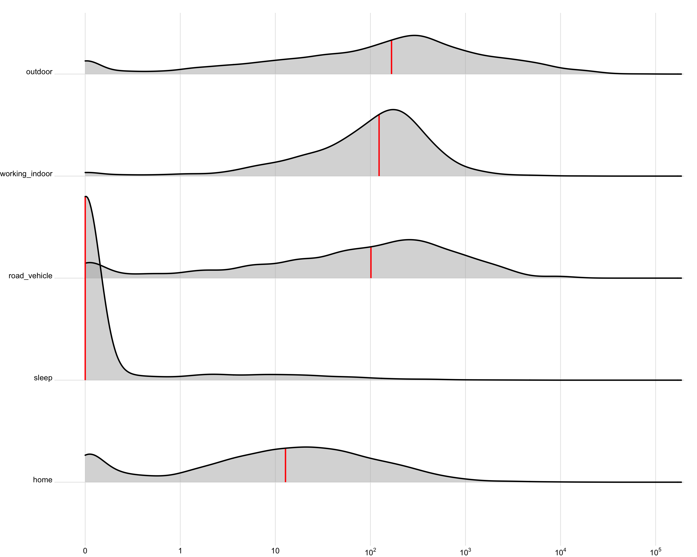
activity_data |>
filter_out(is.na(activity)) |>
site_conv_mutate(rev = FALSE) |>
ggplot(aes(x=geo.MEDI)) +
geom_density_ridges(aes(y=activity),
linewidth = 1, colour = NA,
alpha = 0.5,
from = 0,
) +
geom_density_ridges(aes(y=activity), fill = NA,
alpha = 1, linewidth = 1,
quantile_lines = TRUE, quantiles = 2, vline_color = "red",
linetype = 1,
from = 0,
) +
# scale_fill_manual(values = melidos_colors) +
scale_alpha_continuous(range = c(0, 1)) +
scale_x_continuous(trans = "symlog", breaks = c(0, 10^(0:5)),
labels = expression(0, 1, 10, 10^2, 10^3, 10^4, 10^5)) +
# scale_color_manual(values = melidos_colors) +
guides(fill = "none", color = "none") +
labs(y = NULL, x = NULL) +
theme_ridges() +
coord_cartesian(xlim = c(0, 10^5)) +
theme_sub_plot(margin = margin(r = 20, t = 20)) +
theme_sub_axis_left(text = element_text(vjust = 0))
```
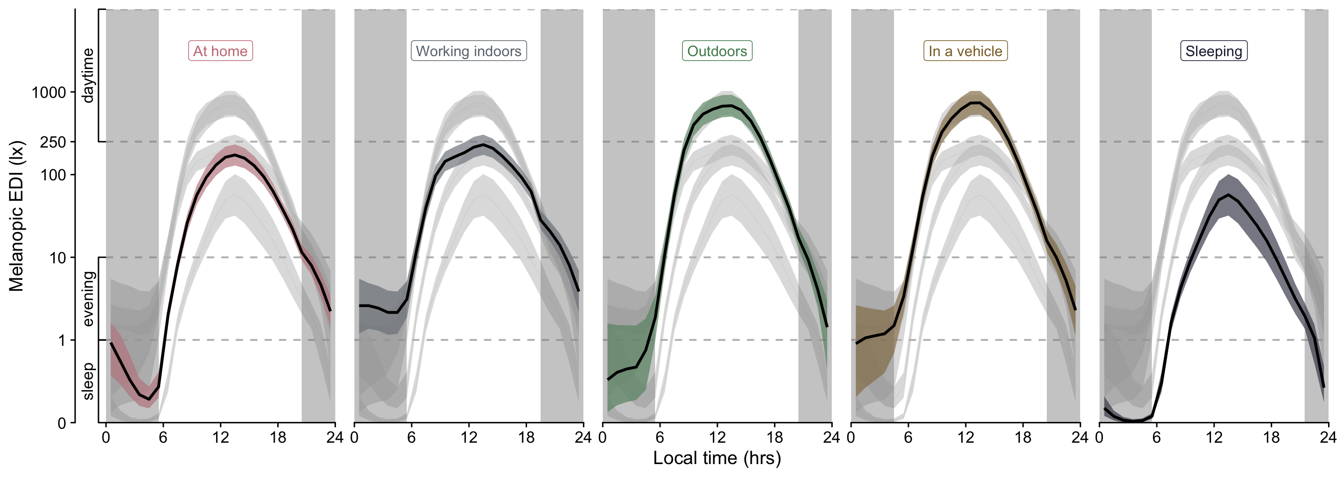
### Interpretation
- Overall, an average mel EDI of about 60 lx (based on geometric mean) is reached with `awake at home`. This value somewhat varies between sites, with The Netherlands, Dortmund, and Sweden, achieving substantially higher values (factor 2.35, 2.03, and 1.76, respectively). They nevertheless do not reach recommended values of 250lx during the day. Tübingen, Germany, and Ghana reach substantially lower values (factor 0.46 and 0.32 respectively).
- When `Sleeping in bed`, about 4% of the mel EDI can be achieved on average (2.3936). There is very high variance between the different sites, with factor ranging between 44% of that value (Tübingen, Germany) to 757% (The Munich).
- When people are `On the road`, they achieve about 4.88 times more light compared to `at home` (292 lx). Dortmund, Germany, achieves still higher values (times 2.04), while Tübingen, Germany has only about one third (0.35).
- `Working indoors` increases the melanopic EDI by a factor of 3.23 (193 lx). The Netherlands and Sweden reach higher levels still (1.8 and 1.79, respectively), while Tübingen, Germany, and Ghana see lower levels of increase (0.57 and 0.62, respectively).
- `Outdoors` translates to about x8.82 the amount of light levels compared to `at home` (~528 lx). Values are similar across sites, with three notable exceptions: Sweden and The Netherlands have significantly higher values still (3.33 and 2.24, respectively), while Munich, Germany sees much lower values (0.23).
- Overall, the effect of self-reported activity is large - 62% of variance can be explained simply through those categories. While site and interindividual differences are significant, they contribute considerably less (9% each). In summary, activity is a good, albeit worse predictor compared to self-reported light source
### Co-occurance of light and activity
```{r}
activity_data |>
  count(activity, lightsource_primary) |>
  pivot_wider(names_from = activity, values_from = n) |>
  drop_na() |>
  gt()
```
As can be seen by the cross-table, the two variables are strongly correlated. However, some differentiating potential lies e.g., in the home and working indoor activity, that provides a very even split between electric light indoors, daylight indoors, and emissive display light. Similarly, daylight outdoors can be split between outdoor and on the road activities.
### Exploration: GAM of activity x time
In this exploratory analysis, we study the nonlinear effect of time on the type of activity, based on the final model from RQ1:
```{r}
#| filename: Prepare GAM data
GAM_data <-
  hourly_data2 |>
  ungroup() |>
  select(site, Id, Datetime, MEDI, photoperiod.state, Date, dawn, dusk, starts_with("act_")) |>
  pivot_longer(cols = starts_with("act_"), names_to = "activity", names_prefix = "act_", values_to = "value") |>
  add_Time_col() |>
  mutate(activity =
           fct(activity) |>
           fct_collapse(outdoor = c("free_outdoor", "working_outdoor", "road_open")) |>
           fct_recode(NULL = "other") |>
           fct_relevel("home")
         ) |>
  drop_na(activity) |>
  filter(value) |>
  distinct(.keep_all = TRUE, site, Id, Datetime, activity) |>
  ungroup() |>
  mutate(Time = as.numeric(Time)/3600 + 0.5,
         across(c(site, Id, photoperiod.state,
                  activity, Date),
                factor),
         Id_date = interaction(Id, Date),
         lzMEDI = log_zero_inflated(MEDI),
         photoperiod = (dusk - dawn) |> as.numeric()
  ) |>
  group_by(Id) |>
  mutate(AR.start = ifelse(row_number() == 1, TRUE, FALSE))

H4_form_gam <- lzMEDI ~ s(Time, k = 12) + s(Time, activity, bs = "sz", k = 12) + s(Time, site, bs = "sz", k = 12) + s(Time, photoperiod.state, bs = "sz", k=12) + s(Time, Id, bs = "fs") + s(Id_date, bs = "re")
```
```{r}
#| filename: Main model
H4_model_gam <-
  bam(H4_form_gam,
      data = GAM_data,
      discrete = TRUE,
      method = "fREML",
      nthreads = 10
      )

r1 <- start_value_rho(H4_model_gam,
                      plot=TRUE)
H4_model_gam <-
bam(H4_form_gam,
data = GAM_data,
discrete = TRUE,
method = "fREML",
nthreads = 10,
rho = r1,
AR.start = AR.start
)
acf_resid(H4_model_gam, split_pred = "AR.start")
H4_summary_gam <- summary(H4_model_gam)
H4_summary_gam
H4_model_gam |> glance()
H4_model_gam |> appraise()
```
```{r}
#| filename: Variance explained
Xp <- predict(H4_model_gam, type = "terms")
variance <- apply(Xp, 2, var)
cor(Xp)
H4_R2 <- (variance/sum(variance)) |> enframe(value = "R2", name = "parameter")
H4_R2
```
```{r}
#| filename: Null model
H2_model_gam <-
  bam(H2_form_gam,
      data = GAM_data,
      discrete = TRUE,
      method = "fREML",
      nthreads = 10
      )

r1 <- start_value_rho(H2_model_gam,
                      plot=TRUE)
H2_model_gam <-
bam(H2_form_gam,
data = GAM_data,
discrete = TRUE,
method = "fREML",
nthreads = 10,
rho = r1,
AR.start = AR.start
)
acf_resid(H2_model_gam, split_pred = "AR.start")
```
```{r}
AIC(H4_model_gam, H2_model_gam)
```
```{r}
H4_model_gam |> draw(select = "s(Time,activity)")
H4_model_gam |> draw(select = "s(Time)")
```
####Visualization
```{r}
#| filename: prepare lightsource model H4 plot
H4_act_data <-
H4_model_gam |>
  conditional_values(
    condition = list(Time = seq(0.5, 23.5, by = 1), "activity", "photoperiod.state"),
    exclude = c("s(Time,Id)", "s(Id_date)", "s(Time,site)")
    ) |>
  mutate(across(c(.fitted, .lower_ci, .upper_ci),
                exp_zero_inflated)
  )

H4_act_data <-
GAM_data |>
  Datetime2Time() |>
  group_by(activity, Time) |>
  summarize(
    .groups = "drop_last",
    dawn = dawn |> as.numeric() |> mean(na.rm = TRUE)/3600,
    dusk = dusk |> as.numeric() |> mean(na.rm = TRUE)/3600,
    n = n()
  ) |>
  mutate(
    photoperiod.state = ifelse(between(Time, dawn, dusk), "day", "night")
  ) |>
  select(-c(dawn, dusk)) |>
  left_join(H4_act_data, by = c("activity", "Time", "photoperiod.state"))

H4_act_data_phot <-
H4_act_data |>
  number_states(photoperiod.state) |>
  filter(photoperiod.state == "night") |>
  group_by(activity, photoperiod.state.count) |>
  summarize(xmin = min(Time),
            xmax = max(Time),
            .groups = "drop_last") |>
  mutate(across(c(xmin, xmax), \(x) replace_values(x,
                                                   0.5 ~ 0,
                                                   23.5 ~ 24)))
```
```{r}
#| filename: Visualize lightsource model H4
#| fig-height: 5
#| fig-width: 14

act_labels <-
  tibble(
    level = c("home", "working_indoor", "outdoor", "road_vehicle", "sleep"),
    label = c("At home", "Working indoors", "Outdoors", "In a vehicle", "Sleeping")
  )

act_colors <-
  c(
    `Working indoors` = "#6C757D", # slate gray
    `At home` = "#C97B84",         # muted rose
    `In a vehicle` = "#8C6D31",    # brown/bronze
    Outdoors = "#4F8A5B",          # muted forest green
    Sleeping = "#1B1F3B"           # dusty indigo
  )

H4_pred <-
H4_act_data |>
  mutate(activity = factor(activity, levels = act_labels$level, labels = act_labels$label)) |>
  ggplot(aes()) +
  map(c(1,10,250, 10^4),
          \(x) geom_hline(aes(yintercept = x),
                          col = "grey", linetype = "dashed")
      ) +
  geom_rect(data = H4_act_data_phot |>
  mutate(activity = factor(activity, levels = act_labels$level, labels = act_labels$label)) ,
            aes(xmin = xmin, ymin = -Inf, ymax = Inf, xmax = xmax),
            alpha = 0.25, inherit.aes = FALSE) +
  geom_ribbon(aes(x = Time, ymin = .lower_ci,
                  ymax = .upper_ci, fill = activity), alpha = 0.5) +

  geom_line(aes(x = Time, y = .fitted,
                col = activity), linewidth = 0.1) +
  geom_line(aes(x = Time, y = .fitted), linewidth = 1) +
  scale_fill_manual(values = act_colors) +
  scale_color_manual(values = act_colors) +
  theme_cowplot() +
  scale_y_continuous(trans = "symlog", breaks = c(0,1,10,100,250, 1000)) +
  scale_x_continuous(breaks = seq(0, 24, by = 6)) +
  coord_cartesian(xlim = c(0,24), ylim = c(0,10^4), expand = FALSE) +
  labs(y = "Melanopic EDI (lx)", x = "Local time (hrs)", fill = "Primary lightsource", col = "Primary lightsource") +
  facet_wrap(~activity, nrow = 1) +
  guides( y = guide_axis_stack(Brown_bracket, "axis")) +
  gghighlight(
    label_key = activity,
    label_params = list(x = 12, y = 4.5, force = 0, hjust = 0.5)
  ) +
  # geom_text(aes(label = paste0("|", n, "|"), x = Time, y = 7000), size = rel(1.5)) +
  theme_sub_strip(background = element_blank(),
                  text = element_blank()) +
  theme(panel.spacing = unit(1, "lines"),
        plot.caption = element_textbox_simple())
  # labs(caption = Brown_caption)
H4_pred
```
```{r}
#| filename: Visualize model terms
Term_data <-
  H4_act_data |> select(Time, activity) |>
  left_join(
    H4_model_gam |>
  smooth_estimates(select = "s(Time,activity)", n=24),
  by = c("Time", "activity")
  ) |>
  ungroup() |>
  complete(Time, activity) |>
  mutate(.lower_ci = .estimate -1.96*.se,
         .upper_ci = .estimate +1.96*.se,
         .fitted = .estimate,
         signif = .lower_ci > 0 | .upper_ci < 0,
         signif_id = consecutive_id(signif),
         .by = activity) |>
    mutate(activity = factor(activity, levels = act_labels$level, labels = act_labels$label))

P_terms <-
Term_data |>
  ggplot(aes()) +
  map(c(log10(c(0.1, 0.2, 0.5, 2, 5, 10))),
      \(x) geom_hline(yintercept = x, linewidth = 0.5, col = "grey", linetype = 2)) +
  geom_rect(data = H4_act_data_phot |>
              mutate(activity = factor(activity, levels = act_labels$level, labels = act_labels$label)),
            aes(xmin = xmin, ymin = -Inf, ymax = Inf, xmax = xmax),
            alpha = 0.25, inherit.aes = FALSE) +
  geom_ribbon(aes(x = Time, ymin = .lower_ci,
                  ymax = .upper_ci, fill = activity),
              alpha = 0.5) +
  geom_hline(yintercept = 0, linewidth = 1, linetype = 2) +
  geom_line(aes(x = Time, y = .fitted),
            linewidth = 1) +
  geom_line(data = \(x) filter(x, signif),
            aes(x = Time, y = .fitted, group = signif_id),
            col = "red", linewidth = 1) +
  scale_fill_manual(values = act_colors) +
  # scale_color_manual(values = c(melidos_colors)) +
  theme_cowplot() +
  scale_y_continuous(labels = expression(10^-1, 5^-1, 2^-1, "1  ", "2  ", "5  ", "10  "),
                     breaks = log10(c(0.1, 0.2, 0.5, 1, 2, 5, 10)))+
  scale_x_continuous(breaks = seq(0, 24, by = 6)) +
  coord_cartesian(xlim = c(0,24), expand = FALSE) +
  guides(fill = "none") +
  labs(y = "Factor", x = "Local time (hrs)", fill = "Primary lightsource") +
  facet_wrap(~activity, nrow = 1) +
  theme_sub_strip(background = element_blank(),
                  text = element_blank()) +
  theme(panel.spacing = unit(1, "lines"),
        plot.caption = element_textbox_simple())
P_terms
```
```{r}
n_plot_H4 <-
GAM_data |>
  ungroup() |>
  count(Time, activity) |>
      mutate(activity = factor(activity, levels = act_labels$level, labels = act_labels$label)) |>
  ggplot(aes(x=Time)) +
  geom_col(aes(y=n, fill = activity)) +
  facet_wrap(~activity, nrow = 1) +
  theme_cowplot() +
  scale_fill_manual(values = act_colors) +
  theme_sub_strip(background = element_blank(),
                  text = element_blank()) +
  theme(panel.spacing = unit(1, "lines"),
        plot.caption = element_textbox_simple()) +
  guides(fill = "none") +
  # scale_y_continuous(trans = "symlog", breaks = c(0, 1, 10, 100, 500)) +
  scale_x_continuous(breaks = seq(0, 24, by = 6))
```
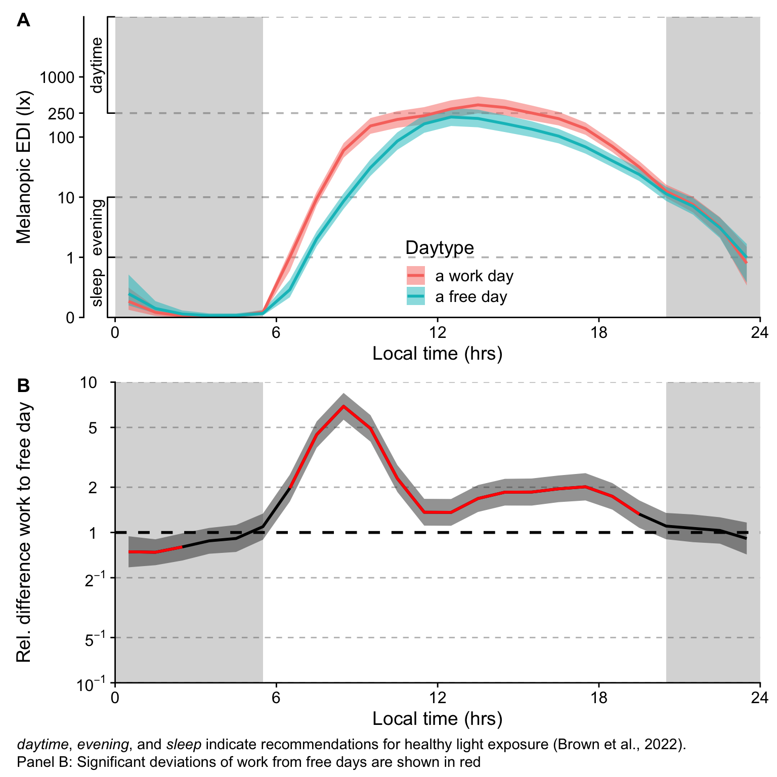
```{r}
#| fig-height: 10
#| fig-width: 15
#| filename: Combination of partial plots H4

H4_pred / P_terms / n_plot_H4 + plot_layout(heights = c(2,2,1)) +
  plot_annotation(tag_levels = "A",
                  caption = paste(Brown_caption,
                                  "Panel B: Significant deviations from the average are shown in red", sep = "<br>"),
                  theme =
                    theme(plot.caption = element_textbox_simple(size = rel(1.5))
                          )
                  )
ggsave("figures/Fig10.pdf", height = 10, width = 15)
ggsave("figures/Fig10.png", height = 10, width = 15)
```
## Hypothesis 5
Hypothesis 5 states:
> There is a significant relationship between LEBA-factors and pre-selected personal light exposure metrics.
*Type of model:* Correlation matrix + LM
*Base formula:* $\text{LEBA factor} \sim \text{Site})$
*False-discovery-rate correction:*
- 4 leba factors x 17 metrics: n = 68
### Preparation
```{r}
#| filename: Collect LEBA data
leba <- load_data("leba") |> flatten_data() |> select(site, Id, leba_f2:leba_f5)
leba_labels <-
leba |> extract_labels() |> enframe() |> filter(str_detect(name, "leba_f.$"))
```
```{r}
#| filenmae: Collect light exposure metrics
load("data/H1_results.RData")
metrics <- metrics |> select(name, type, metric_type, data, engine, response, family, H1_1_sig, H1_lat_sig, H1_phot_sig)
metrics_leba <-
  metrics |>
  filter_out(is.na(response)) |>
  mutate(
    data =
      map(data,
          \(x) x |>
            group_by(site, Id) |>
            summarize(metric = mean(metric, na.rm = TRUE), .groups = "drop_last") |>
            left_join(leba, by = c("site", "Id")) |>
            pivot_longer(leba_f2:leba_f5, names_to = "leba")
          )
  ) |>
  select(name, type, metric_type, data) |>
  unnest(data)
```
### Analaysis
```{r}
#| filename: Test whether sites vary in their leba factors

# test <-
leba |>
  mutate(Id = fct(Id),
         site = fct(site)) |>
  summarize(across(leba_f2:leba_f5,
                    \(x) {
                      data <- pick(cur_column(), site)
                      lm(x~ site, data = data) |> list()
                         }
                    )
                ) |>
  pivot_longer(everything()) |>
  mutate(marginals = map(value, \(x) emmeans(x, ~ site)),
         test = map(marginals, \(x)  joint_tests(x) |> as.tibble()),
         contrasts = map(marginals, contrast)) |>
  unnest(test) |>
  mutate(p.value = p.adjust(p.value, "fdr", n=4),
         signif = p.value <= sig.level) |>
  filter(signif) |>
  select(-p.value) |>
  mutate(contrasts = map(contrasts, as.tibble)) |>
  unnest(contrasts) |>
  filter(p.value <= sig.level) |>
  select(name, contrast, estimate, SE, df, p.value, signif) |>
  gt() |>
  fmt_number() |>
  fmt(p.value, fns= style_pvalue) |>
  tab_header("Significant differences in LEBA factors dependent on sites")
```
Only two factors are significantly different: F2 and F5. Of those, only UCR for F2 and BAUA for F5 show significant differences from the mean, both being 2-3 points lower (post-hoc test). Thus, we deem that the factors can be analysed independent of site.
```{r}
#| filename: create correlation data
H5_corr_matrix <-
  metrics_leba |>
  group_by(name, leba) |>
  drop_na(metric, value)

H5_n <- n_groups(H5_corr_matrix)

H5_corr_matrix <-
H5_corr_matrix |>
  summarize(
      correlation = cor(metric, value, method = "spearman"),
              p_value = cor.test(metric, value)$p.value |>
                        p.adjust(method = "fdr", n = H5_n),
              significant = p_value <= sig.level,
              .groups = "drop") |>
  mutate(
    name = name |> str_replace_all("_", " ") |> str_to_sentence(),
    labels = replace_values(leba, from = leba_labels$name, to = leba_labels$value) |>
      fct() |> fct_rev()
  )
```
#### Visualization
```{r}
#| filename: Visualize correlation matrix
#| fig-width: 12
#| fig-height: 5

H5_corr_matrix |>
  ggplot(aes(x = name, y = labels, fill = abs(correlation))) +
  geom_blank() +
  geom_tile(data = H5_corr_matrix |> filter(significant), linewidth = 0.25) +
  geom_text(
    aes(label =
          paste(
            paste("r=",round(correlation, 2)),
            p_value %>% style_pvalue(prepend_p = TRUE),
            sep = "\n"),
        color = significant
        ),
    fontface = "bold",
    size = 1.8) +
  coord_fixed() +
  scale_fill_viridis_c(limits = c(0,1))+
  guides(color = "none", fill = "none")+
  scale_color_manual(values = c("red2", "white"), drop = FALSE)+
  labs(y = "LEBA factors", x = "Metrics",
       fill = "(abs) Correlation")+
  theme(axis.text.x = element_text(angle = 45, hjust = 1)) +
  labs(caption = paste0("p-values are fdr-corrected for n= ", H5_n, " comparisons"))
ggsave("figures/Fig6.pdf", width = 12, height = 5)
ggsave("figures/Fig6.png", width = 12, height = 5)
```
### Interpretation
- There is no overarching corelation between light exposure metrics and LEBA factors. We do find a significant correlation of Dose and Duration above 1000 for `F2: Spending time outdoors`, which makes sense from a theoretical point of view (spending more time outside would yield in a higher dose and duration in daylight levels). These correlations are small in size and only explain a small amount of variance. Dose: $r=0.27, R^2=0.07, p=0.013$; Duration above 250 lx melanopic EDI: $r=0.29, R^2=0.08, p=0.032$
## Hypothesis 6
### Details
Hypothesis 6 states:
> There is a significant relationship between the day type, daily exercise, and sleep with the hourly geometric mean of light exposure
*Type of model:* GLMM
*Base formula:*
- $\text{mel EDI} \sim \text{day type}*\text{Site} + \text{daily exercise}*\text{Site} + \text{sleep duration}*\text{Site} +(1|\text{Participant})$
*Notes:*
- The confirmatory tests look at the base model compared to the Null models for each covariate
- Site was sum-coded, so as to calculate an average effect of site
- Sleep duration is based on the previous night
*Specific formulas:*
- $\text{Metric} \sim \text{daily exercise}*\text{Site} + \text{sleep duration}*\text{Site}+ (1|\text{Participant})$ (Null model day type)
- $\text{Metric} \sim \text{day type}*\text{Site} + \text{sleep duration}*\text{Site}+ (1|\text{Participant})$ (Null model exercise)
- $\text{Metric} \sim \text{day type}*\text{Site} + \text{daily exercise}*\text{Site} + (1|\text{Participant})$ (Null model sleep duration)
*False-discovery-rate correction:*
- 3 main effects: n=3; site: n=9
### Preparation
```{r}
#| filename: Load other data types
sleep <- load_data("sleepdiaries") |> flatten_data()
exercise <- load_data("exercisediary") |> flatten_data()
sleep <-
sleep |>
mutate(Date = date(wake),
daytype = daytype2 |> fct_relevel("a work day"),
sleep_duration = sleep_duration |> as.numeric()) |>
select(site, Id, Date, sleep_duration, daytype)
exercise <-
exercise |>
select(site, Id, Date, intensity) |>
mutate(intensity = fct_relabel(intensity, \(x) str_extract(x, "^(\\S+)")) |>
fct_relevel("None", "Light", "Moderate")) |>
rename(exercise = intensity)
H6_contextdata <-
full_join(sleep, exercise, by = c("site", "Id", "Date"))
```
```{r}
#| filename: Merge data
H6_data <-
  hourly_data2 |>
  left_join(H6_contextdata, by = c("site", "Id", "Date")) |>
  add_Date_col(Weekday, as.wday = TRUE) |>
  mutate(Weekend = ifelse(as.numeric(Weekday) >5, "Weekend", "Weekday"))
```
```{r}
H6_contextdata <-
  H6_contextdata |>
  mutate(Date = factor(Date))
```
### Testing site-specific differences
```{r}
by.day.data <- H6_contextdata |> mutate(work = daytype == "a work day")
```
```{r}
model_daytype <- glm(work ~ site, data = by.day.data, family = binomial())
summary(model_daytype)
drop1(model_daytype, test = "Chisq")
```
Daytype is not significantly different between sites.
```{r}
model_sleep <- lmer(sleep_duration ~ site + (1|Id), data = by.day.data)
summary(model_sleep)
drop1(model_sleep, test = "Chisq")
```
Sleep duration is not significantly different between sites
```{r}
#check for site differences of exercise:
library(ordinal)
model_exercise_site <- clmm(
  exercise ~ site + (1 | Id),
  data = H6_contextdata
)

summary(model_exercise_site)
drop1(model_exercise_site)
```
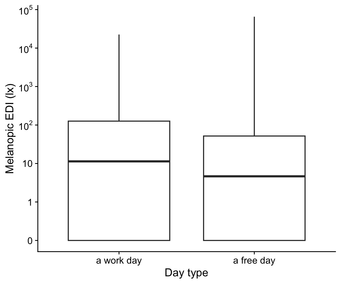
```{r}
#| filename: Plot overview of light against self-reported activity
#| fig-width: 6
#| fig-height: 5
H6_data |>
  drop_na(daytype) |>
  ggplot(aes(x=daytype, y = geo.MEDI)) +
  geom_boxplot() +
  scale_y_continuous(trans = "symlog",
                     breaks = c(0,1,10,100,1000,10000,10^5),
                     labels = expression(0,1,10,10^2,10^3,10^4,10^5)) +
  theme_cowplot() +
  labs(y = "Melanopic EDI (lx)", x = "Day type")
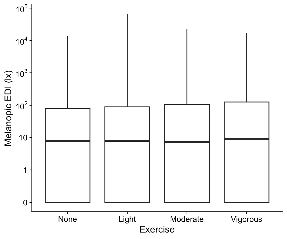
H6_data |>
drop_na(exercise) |>
ggplot(aes(x=exercise, y = geo.MEDI)) +
geom_boxplot() +
scale_y_continuous(trans = "symlog",
breaks = c(0,1,10,100,1000,10000,10^5),
labels = expression(0,1,10,10^2,10^3,10^4,10^5)) +
theme_cowplot() +
labs(y = "Melanopic EDI (lx)", x = "Exercise")
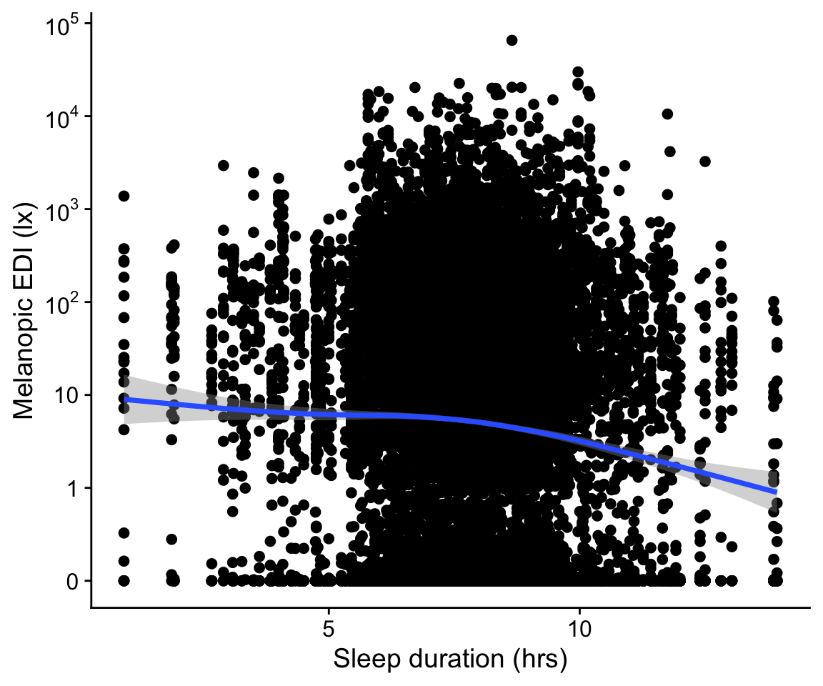
H6_data |>
drop_na(sleep) |>
ggplot(aes(x=sleep_duration, y = geo.MEDI)) +
geom_point() +
geom_smooth() +
scale_y_continuous(trans = "symlog",
breaks = c(0,1,10,100,1000,10000,10^5),
labels = expression(0,1,10,10^2,10^3,10^4,10^5)) +
theme_cowplot() +
labs(y = "Melanopic EDI (lx)", x = "Sleep duration (hrs)")
```
### Analysis
```{r}
#| filename: Fit the model for H6
#| fig-height: 10
#| fig-width: 8
H6_formula_1 <- geo.MEDI ~ site*daytype + site*exercise + site*sleep_duration + (1| Id)
H6_formula_0_daytype <- geo.MEDI ~ site*exercise + site*sleep_duration + (1| Id)
H6_formula_0_exercise <- geo.MEDI ~ site*daytype + site*sleep_duration + (1|Id)
H6_formula_0_sleep <- geo.MEDI ~ site*daytype + site*exercise + (1|Id)
H6_formula_0_site <- geo.MEDI ~ daytype + exercise + sleep_duration + (1|Id)

#confirmatory
H6_model_1 <-
  glmmTMB(H6_formula_1,
          data = H6_data |> drop_na(geo.MEDI, daytype, exercise, sleep_duration),
          REML = FALSE,
          family = tweedie(),
          contrasts = list(site = "contr.sum")
          )
H6_model_0_daytype <-
  glmmTMB(H6_formula_0_daytype,
          data = H6_data |> drop_na(geo.MEDI, daytype, exercise, sleep_duration),
          REML = FALSE,
          family = tweedie(),
          contrasts = list(site = "contr.sum")
          )
H6_model_0_exercise <-
  glmmTMB(H6_formula_0_exercise,
          data = H6_data |> drop_na(geo.MEDI, daytype, exercise, sleep_duration),
          REML = FALSE,
          family = tweedie(),
          contrasts = list(site = "contr.sum")
          )
H6_model_0_sleep <-
  glmmTMB(H6_formula_0_sleep,
          data = H6_data |> drop_na(geo.MEDI, daytype, exercise, sleep_duration),
          REML = FALSE,
          family = tweedie(),
          contrasts = list(site = "contr.sum")
          )
H6_model_0_site <-
  glmmTMB(H6_formula_0_site,
          data = H6_data |> drop_na(geo.MEDI, daytype, exercise, sleep_duration),
          REML = FALSE,
          family = tweedie(),
          # contrasts = list(site = "contr.sum")
          )

comp_daytype <-
anova(H6_model_0_daytype, H6_model_1)
comp_daytype
comp_exercise <-
anova(H6_model_0_exercise, H6_model_1)
comp_exercise
comp_sleep <-
anova(H6_model_0_sleep, H6_model_1)
comp_sleep
AIC(H6_model_0_sleep, H6_model_0_exercise, H6_model_0_daytype, H6_model_1) |>
arrange(AIC) |>
rownames_to_column("model") |> gt()
```
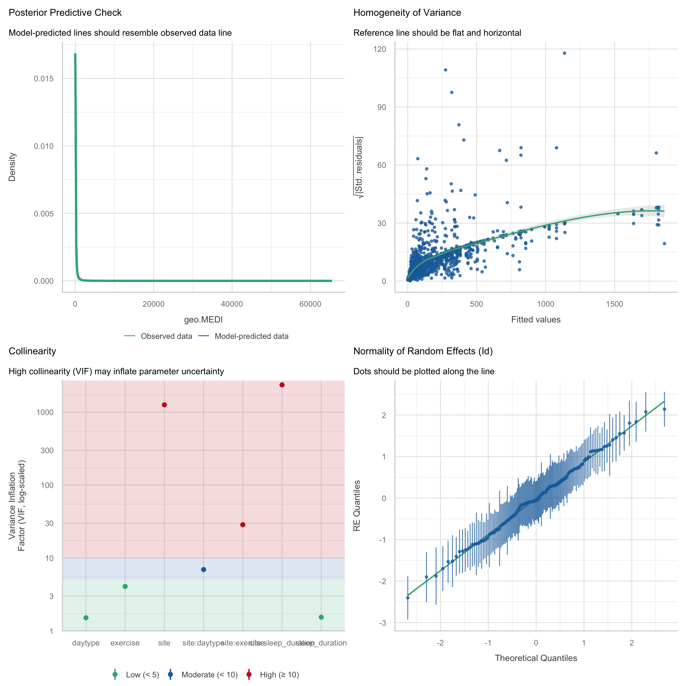
Both AIC and ∆loglik comparisons suggest that the full interaction model is the most relevant one.
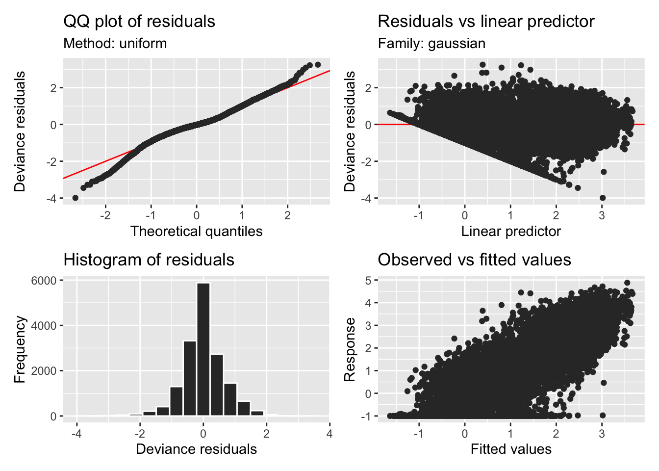
```{r}
#| fig-width: 12
#| fig-height: 12
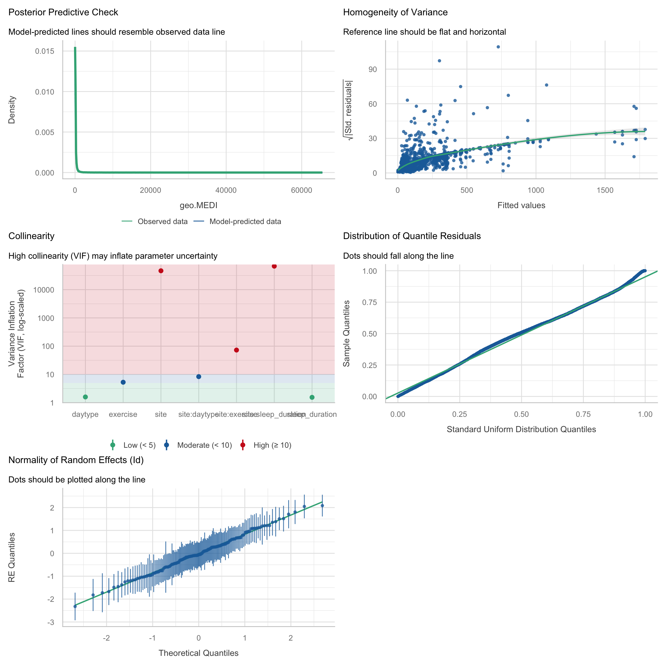
check_model(H6_model_1)
```
```{r}
tab_model(H6_model_1, CSS = css_theme("cells"))
```
```{r}
H6_r2_1 <- r2_helper(H6_model_1, H6_data, tweedie(), "geo.MEDI", "(1 | Id)")
H6_r2_0_daytime <- r2_helper(H6_model_0_daytype, H6_data, tweedie(), "geo.MEDI", "(1 | Id)")
H6_r2_0_exercise <- r2_helper(H6_model_0_exercise, H6_data, tweedie(), "geo.MEDI", "(1 | Id)")
H6_r2_0_sleep <- r2_helper(H6_model_0_sleep, H6_data, tweedie(), "geo.MEDI", "(1 | Id)")
H6_r2_0_site <- r2_helper(H6_model_0_site, H6_data, tweedie(), "geo.MEDI", "(1 | Id)")
H6_tab_r2 <-
  tribble(
    ~type, ~r2,
    "Model", H6_r2_1$R2_conditional,
    "All fixed", H6_r2_1$R2_marginal,
    "Residual", 1-H6_r2_1$R2_conditional,
    "Daytype", H6_r2_1$R2_marginal - H6_r2_0_daytime$R2_marginal,
    "Exercise", H6_r2_1$R2_marginal - H6_r2_0_exercise$R2_marginal,
    "Sleep", H6_r2_1$R2_marginal - H6_r2_0_sleep$R2_marginal,
    "Random", H6_r2_1$R2_conditional - H6_r2_1$R2_marginal,
    "Site", H6_r2_1$R2_marginal - H6_r2_0_site$R2_marginal,
  ) |>
  mutate(r2= r2 |> round(2))
```
#### Basic table
```{r}
H6_tab_ran <-
  H6_model_1 |>
  tidy() |>
  mutate(signif = p.value <= sig.level,
         estimate = exp(estimate) |> round(2)) |>
  filter(effect == "ran_pars") |>
  select(term, estimate)

H6_tab_reference <-
  H6_model_1 |>
  emmeans(~ daytype + exercise + sleep_duration, type = "response",
          at = list(daytype = "a work day",
                    exercise = "None"
                    )) |>
  as.tibble() |>
  rename(estimate = response)

H6_tab_daytype <-
  H6_model_1 |>
  emmeans(~ daytype, type = "response") |>
  contrast(method = "trt.vs.ctrl") |>
  as.tibble() |>
  rename(estimate = ratio)
H6_tab_exercise <-
  H6_model_1 |>
  emmeans(~ exercise, type = "response") |>
  contrast(method = "trt.vs.ctrl") |>
  as.tibble() |>
  rename(estimate = ratio)
H6_tab_sleep <-
  H6_model_1 |>
  emtrends(~ sleep_duration, var = "sleep_duration", type = "response") |>
  as.tibble() |>
  rename(estimate = sleep_duration.trend) |>
  mutate(p.value = comp_sleep$`Pr(>Chisq)`[2],
         estimate = exp(estimate))
H6_tab_daytype_interaction <-
  H6_model_1 |>
  emmeans(~ site | daytype, type = "response") |>
  contrast() |>
  as.tibble() |>
  rename(estimate = ratio)

H6_tab_exercise_interaction <-
  H6_model_1 |>
  emmeans(~ site | exercise, type = "response") |>
  contrast() |>
  as.tibble() |>
  rename(estimate = ratio)

H6_tab_sleep_interaction <-
  H6_model_1 |>
  emtrends(~ site | sleep_duration, var = "sleep_duration", type = "response") |>
  contrast() |>
  as.tibble() |>
  mutate(estimate = exp(estimate))

H6_tab_fix <-
  bind_rows(H6_tab_reference,
            H6_tab_daytype,
            H6_tab_exercise,
            H6_tab_sleep,
            H6_tab_daytype_interaction,
            H6_tab_exercise_interaction,
            H6_tab_sleep_interaction
            ) |>
  mutate(signif = p.value <= sig.level) |>
  select(-c(df, asymp.LCL, asymp.UCL, null, z.ratio)) |>
  relocate(contrast, .before = 1) |>
  mutate(site = contrast |> as.character(),
         daytype =
           daytype |> as.character() |>
           replace_when(
             str_detect(contrast, "a work day") ~ str_remove(contrast, " / a work day")
           ),
         exercise =
           exercise |> as.character() |>
           replace_when(
             str_detect(contrast, "None") ~ str_remove(contrast, " / None")
           ),
         site = replace_when(site,
                             is.na(site) ~ "Overall",
                             str_detect(site, " effect") ~ str_remove(site, " effect"),
                             str_detect(contrast, "a work day") ~ "Overall",
                             str_detect(contrast, "None") ~ "Overall"),
         sleep = ifelse(is.na(sleep_duration), NA, "sleep"),
         .before = 1

  ) |>
  select(-contrast, -sleep_duration) |>
  pivot_longer(sleep:exercise, names_to = "covariate") |>
    drop_na(value) |>
    filter_out(site == "Overall", value == "sleep", is.na(p.value)) |>
  pivot_wider(id_cols = c(site), names_from = c(covariate, value), values_from = estimate:signif)
```
```{r}
H6_tab <-
H6_tab_fix |>
  site_conv_mutate(rev = FALSE, other.levels = "Overall") |>
  arrange(site) |>
  gt() |>
  cols_label_with(
    fn =
      \(x) str_remove(x, "estimate_") |>
            str_remove("daytype_") |>
            str_remove("sleep_") |>
            str_remove("exercise_") |>
            str_to_sentence()
    )|>
  tab_spanner(
    md(
      paste0("Day type ($p = ",
             comp_daytype$`Pr(>Chisq)`[2] |> style_pvalue(),
             "$, $R^2=", H6_tab_r2$r2[4],
             "$)")
      ),
    columns = contains("daytype_")) |>
  tab_spanner(
    md(
      paste0("Exercise ($p = ",
             comp_exercise$`Pr(>Chisq)`[2] |> style_pvalue(),
             "$, $R^2=", H6_tab_r2$r2[5],
             "$)")
      ),
    columns = contains("exercise_"))|>
      cols_hide((contains(c("p.value_", "signif_")))) |>
      cols_hide((starts_with(c("SE_")))) |>
  sub_missing(missing_text = "") |>
  gt::rows_add(site = NA, .after = 1) |>
  tab_style(
    style = list(css(`padding-top` = "0px",
            `padding-bottom` = "0px"),
            cell_fill("lightgrey")
            ),
locations = cells_body(rows = 2)) |>
  gt_multiple(
    names(H6_tab_fix) |>
      subset(str_detect(names(H6_tab_fix), "estimate_")) |>
      str_remove("estimate_"),
    bold_p.) |>
  tab_style_body(
    style = cell_borders(weight = px(2)),
    rows = 1,
    columns = 2:3,
    fn = \(x) TRUE
  ) |>
    fmt(starts_with("estimate"),
      fns = \(x)
      {x <- x |> gt::vec_fmt_number()
      str_c(x, "×")}
      ) |>
  fmt(columns = 2:3,
      rows = site == "Overall",
      fns = \(x)
      {x <- x |> gt::vec_fmt_number()
      str_c(x, " lx")}
      ) |>
  gt_multiple(
    melidos_colors |> names(),
    style_rows
  ) |>
  tab_style(
    style = cell_text(weight = "bold"),
    locations = list(
      cells_column_labels(),
      cells_column_spanners(),
      cells_body(columns = site),
      cells_body(2:3,1)
    )
  ) |>
  cols_label(
    site = md(paste0("Site<br>($p = ",
             comp_site$`Pr(>Chisq)`[2] |> style_pvalue(),
             "$, $R^2=", H6_tab_r2$r2[8],
             "$)")),
    estimate_sleep_sleep =  md(
      paste0("Sleep<br>($p = ",
             comp_sleep$`Pr(>Chisq)`[2] |> style_pvalue(),
             "$, $R^2=", H6_tab_r2$r2[6],
             "$)")
      )
    ) |>
  tab_header(
    title = "Model results for Hypothesis 6",
    subtitle = H6
  ) |>
  tab_footnote(
    md("Values shown in **bold** are significant at $p<0.05$. False-discovery-rate adjustment for n=3 overall, n=3 in exercise, and n=9 in site")
  ) |>
  cols_width(
             site ~ px(150),
             estimate_sleep_sleep ~ px(150),
             everything() ~ px(100)) |>
    tab_footnote(
    "Reference value, for `A work day` with an average of `7.9 hours of sleep`, and exercise `None`. All other values have to be multiplied by the reference value, their respective `Overall` multiplier, and optionally the site interaction to get the estimated mel EDI for a given combination.", locations = cells_body(2:3,1)
  ) |>
  tab_footnote(
    md(paste0("Conditional (Model) $R^2=",
              H6_tab_r2$r2[1],
              "$, Marginal (Fixed effects) $R^2=",
              H6_tab_r2$r2[2],
              "$, Random effect $R^2=",
              H6_tab_r2$r2[7],
              "$, Residual Variance $R^2=",
              H6_tab_r2$r2[3],
              "$; Random effect of participant: $×",
              H6_tab_ran$estimate[1],
              "$; Model based on ",
              H6_data |> drop_na(geo.MEDI, exercise, daytype, sleep_duration) |> nrow() |> vec_fmt_integer(sep_mark = "'"),
              " participant-hours."
              ))
  )
```
```{r}
H6_tab
gtsave(H6_tab, "tables/H6.png", vwidth = 1200)
gtsave(H6_tab, "tables/H6.docx", vwidth = 1200)
```
#### Visualization
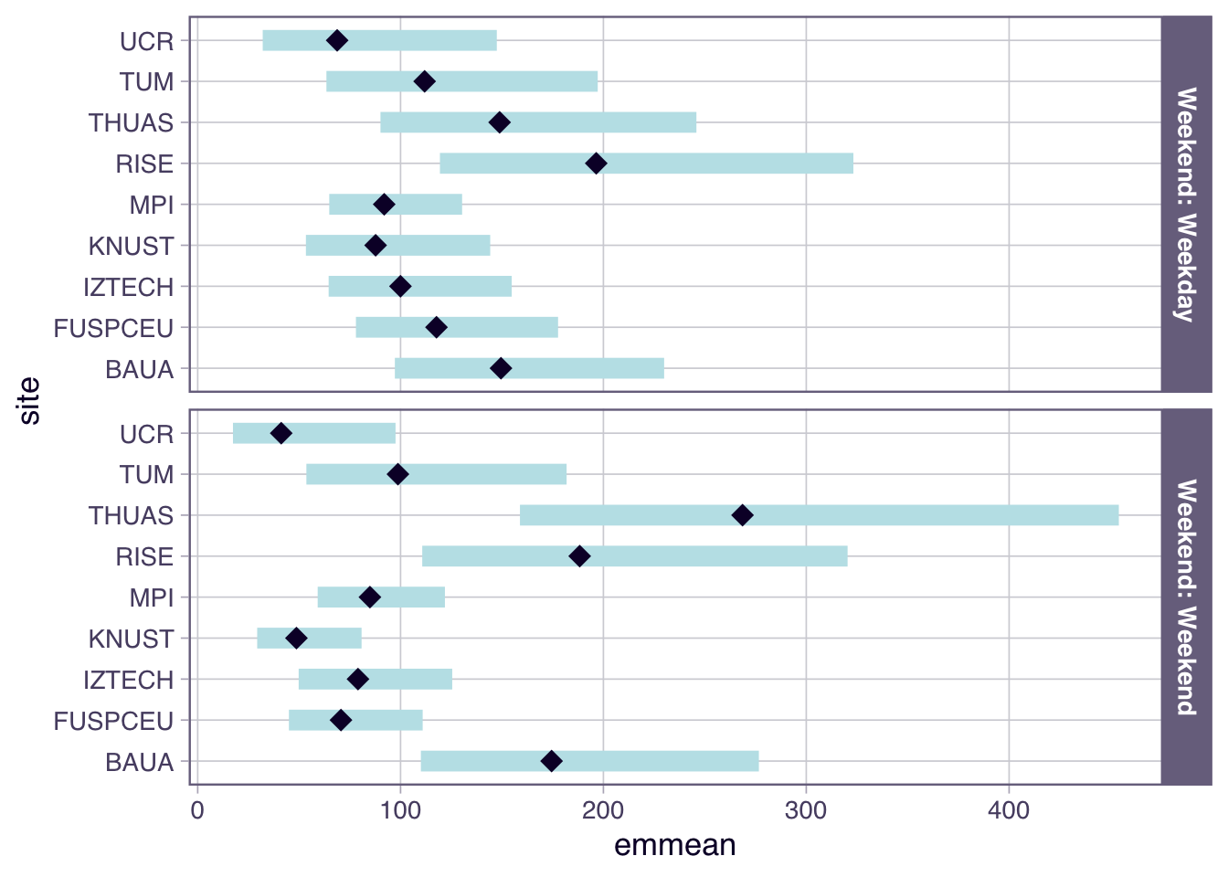
```{r}
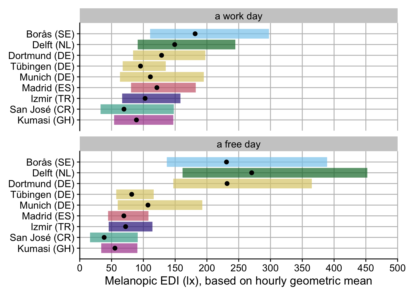
H6_plot <-
H6_model_1 |>
  emmeans(~ site | daytype, type = "response") |>
  plot()

H6_plot <-
  H6_plot$data |>
  as.tibble() |>
  site_conv_mutate(site = pri.fac) |>
    ggplot(
      aes(x = the.emmean, y = pri.fac)
    ) +
    geom_crossbar(aes(xmin = lcl, xmax = ucl, fill = pri.fac), col = NA, alpha = 0.7) +
    geom_point() +
  theme_cowplot() +
  theme(panel.grid.major = element_line(color = "grey")) +
  scale_fill_manual(values = melidos_colors) +
  facet_wrap(~daytype, ncol = 1) +
  scale_x_continuous(breaks = seq(0, 600, by = 50)) +
  coord_cartesian(xlim = c(0, 500), ylim = c(0, 10), expand = FALSE, clip = "off") +
  labs(y = NULL, x = "Melanopic EDI (lx), based on hourly geometric mean") +
    guides(fill = "none") +
  theme(plot.margin = margin(10, 20, 10, 10))

H6_plot
ggsave("figures/Fig_H6.pdf", width = 7, height = 7)
ggsave("figures/Fig_H6.png", width = 7, height = 7)
```
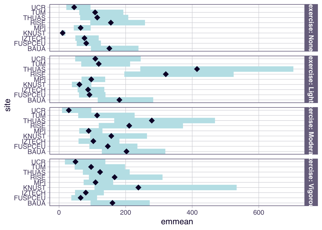
```{r}
H6_model_1 |>
  emmeans(~ site | exercise, type = "response") |>
  plot()
```
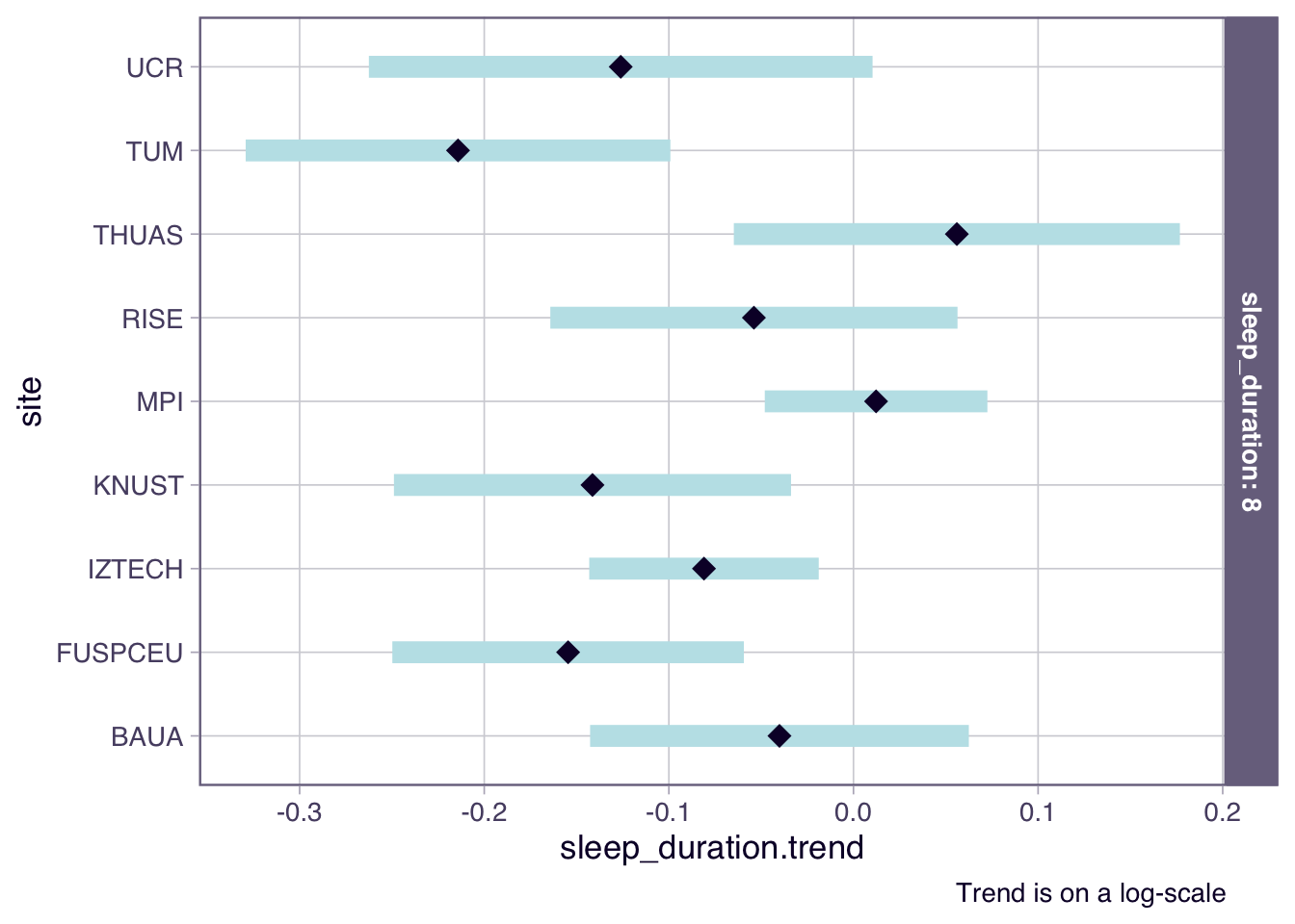
```{r}
H6_model_1 |>
  emtrends(~ site | sleep_duration, var = "sleep_duration", type = "response",
           at = list(sleep_duration = 8)) |>
  plot() +
  labs(caption = "Trend is on a log-scale")
```
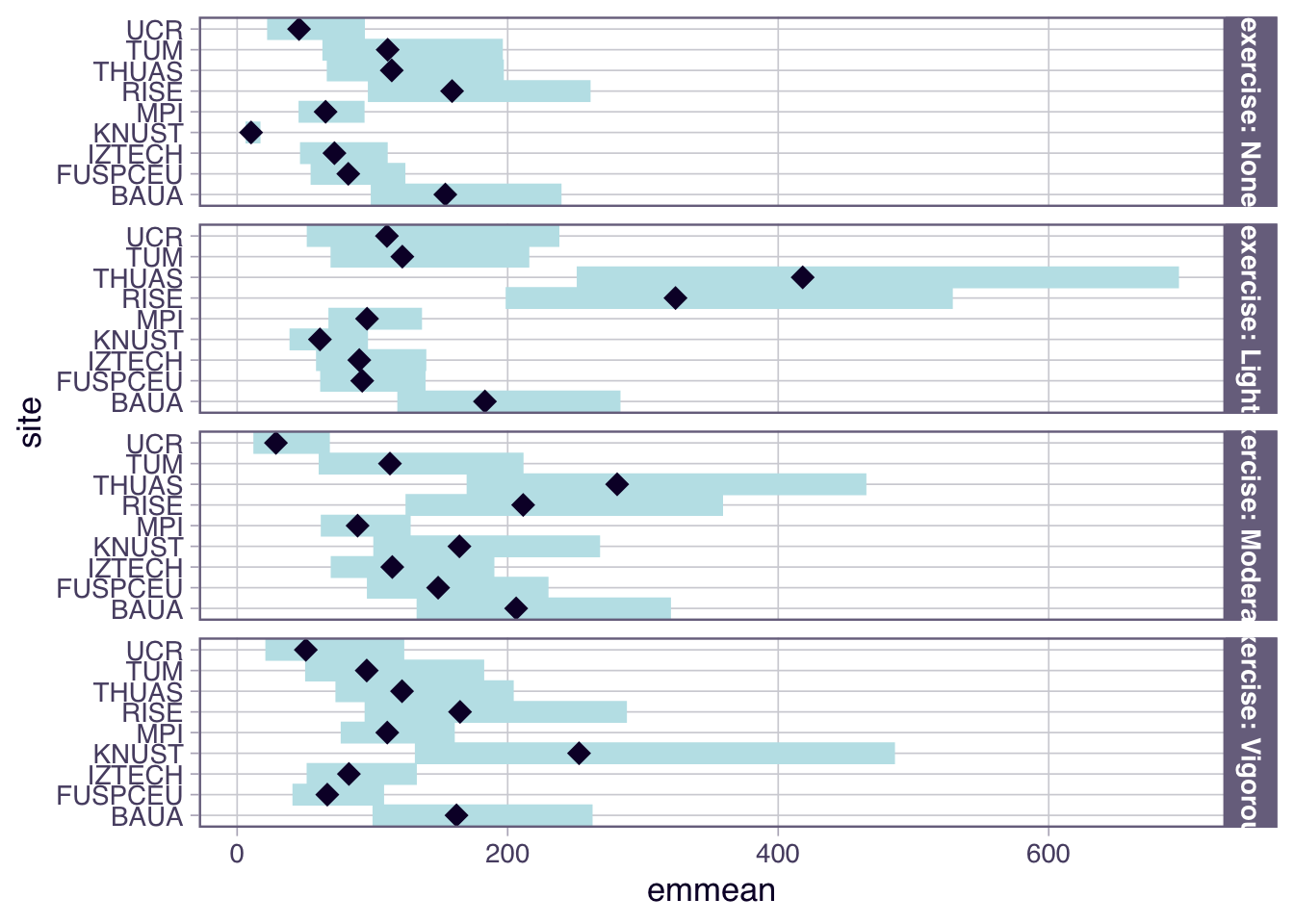
### Interpretation
- While there is no overall difference between work days and free days, Sweden, The Netherlands, and Dortmund, Germany show substantially higher melanopic EDI on free days (factors of 2.22, 2.60, and 2.23, respectively), while Costa Rica and Ghana have substantiall lower values (0.39 and 0.53, respectively).
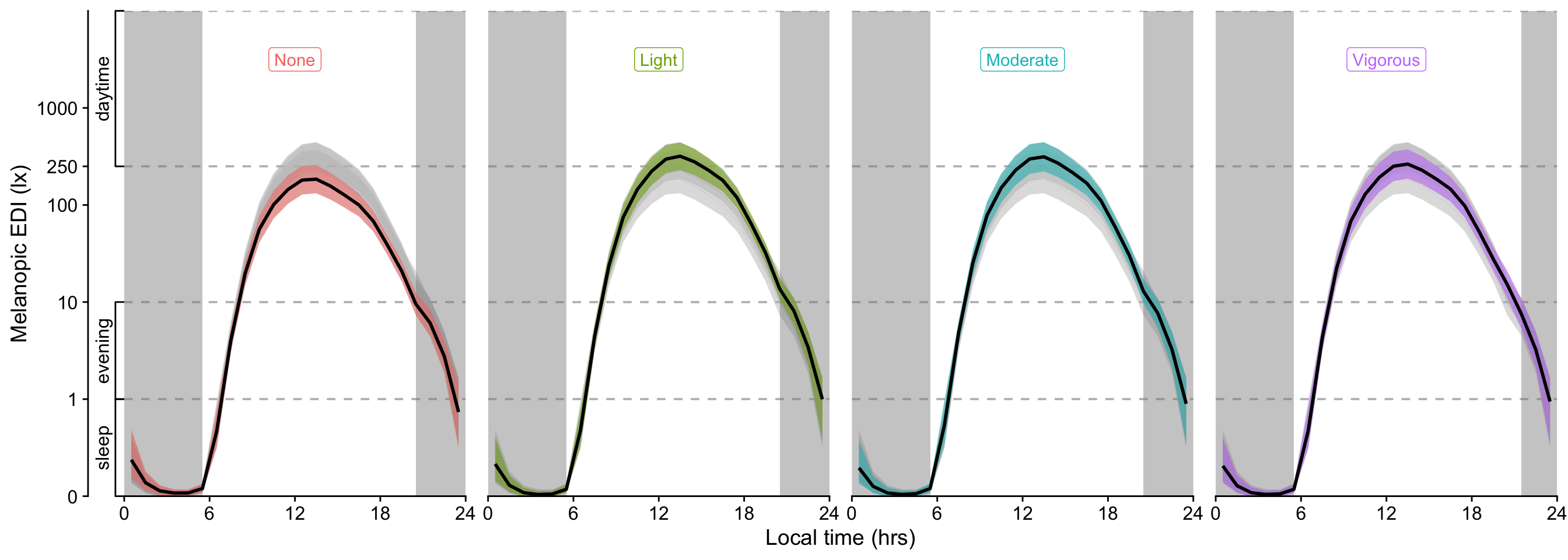
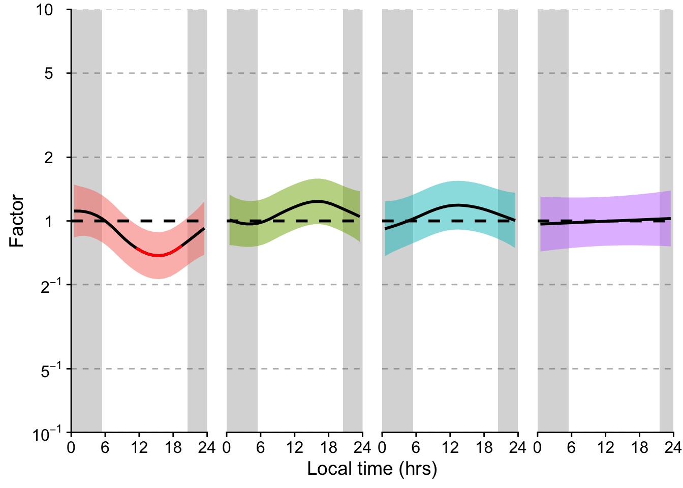
- For exercise, the overall effect is a substantially higher melanopic EDI as long as there is some amount of exercise (>1.50). Sweden and The Netherlands show partially higher values for activity levels below `Vigorous` (>2.14), while Ghana, have very low values for No or light exercise (0.15 and 0.45, respectively), and Costarica has lower values at moderate exercise (0.23)
- There is an overall trend of -8% lower melanopic EDI per additional hour of sleep. Only Tübingen, Germany, shows a flat curve (1.1 x 0.92 = 1.01)
- While all of the effects are significant (at least with their interaction of site), none are very relevant, with unique contributions to $R^2$ values between 0.01 and 0.05
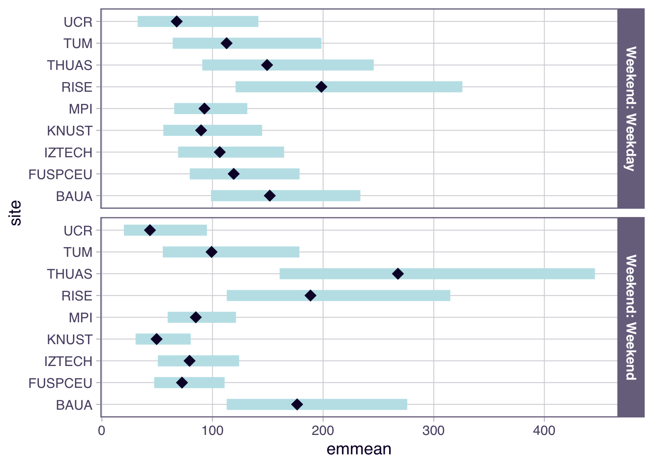
### Weekend instead of free day
This is a quick test to check whether weekend is a better predictor for melanopic EDI.
```{r}
H6_formula_weekend <- geo.MEDI ~ site*Weekend + site*exercise + site*sleep_duration + (1| Id)

H6_model_1_weekend <-
  glmmTMB(H6_formula_weekend,
          data = H6_data |> drop_na(geo.MEDI, daytype, exercise, sleep_duration),
          REML = FALSE,
          family = tweedie(),
          contrasts = list(site = "contr.sum")
          )

AIC(H6_model_1_weekend, H6_model_1)
```
```{r}
H6_model_1_weekend |>
emmeans(~ site | Weekend, type = "response") |>
plot()
```
The quick test shows that daytype is the better predictor compared to weekend (∆AIC), and that the results are broadly the same.
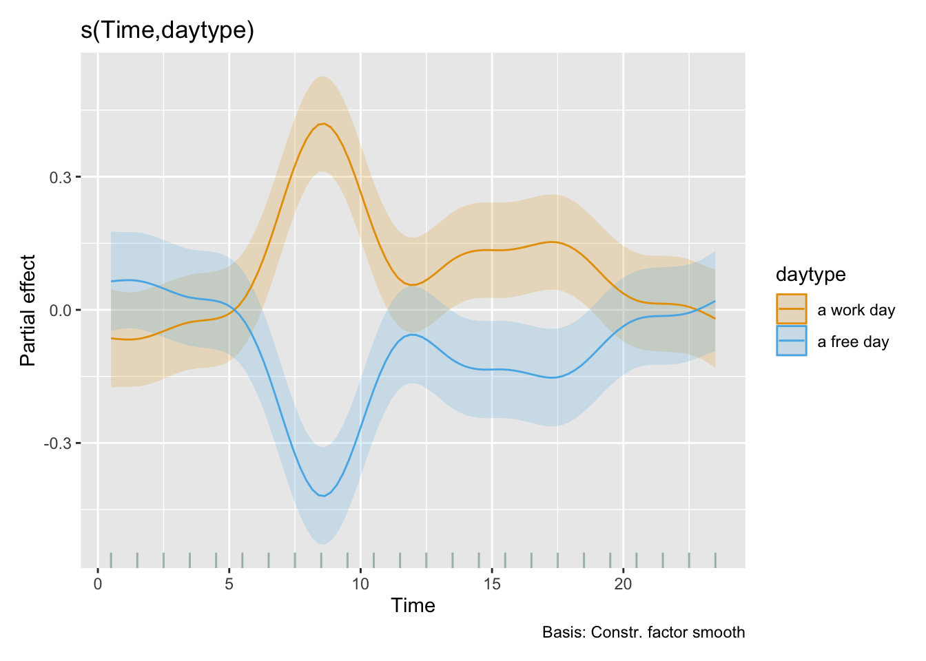
### Exploration: GAM of activity x time
In this exploratory analysis, we study the nonlinear effect of time on the type of activity, based on the final model from RQ1:
```{r}
#| filename: Prepare GAM data
GAM_data <-
H6_data |>
ungroup() |>
select(site, Id, Datetime, MEDI, photoperiod.state, Date, dawn, dusk, exercise, daytype) |>
add_Time_col() |>
drop_na(exercise, daytype) |>
ungroup() |>
mutate(Time = as.numeric(Time)/3600 + 0.5,
across(c(site, Id, photoperiod.state,
Date),
factor),
Id_date = interaction(Id, Date),
lzMEDI = log_zero_inflated(MEDI),
photoperiod = (dusk - dawn) |> as.numeric()
) |>
group_by(Id) |>
mutate(AR.start = ifelse(row_number() == 1, TRUE, FALSE))
H6_form_gam <- lzMEDI ~ s(Time, k = 12) + s(Time, daytype, bs = "sz", k = 12) + s(Time, exercise, bs = "sz", k = 12) + s(Time, site, bs = "sz", k = 12) + s(Time, photoperiod.state, bs = "sz", k=12) + s(Time, Id, bs = "fs") + s(Id_date, bs = "re")
```
```{r}
#| filename: Main model
H6_model_gam <-
bam(H6_form_gam,
data = GAM_data,
discrete = TRUE,
method = "fREML",
nthreads = 10
)
r1 <- start_value_rho(H6_model_gam,
plot=TRUE)
H6_model_gam <-
bam(H6_form_gam,
data = GAM_data,
discrete = TRUE,
method = "fREML",
nthreads = 10,
rho = r1,
AR.start = AR.start
)
acf_resid(H6_model_gam, split_pred = "AR.start")
H6_summary_gam <- summary(H6_model_gam)
H6_summary_gam
H6_model_gam |> glance()
H6_model_gam |> appraise()
```
```{r}
#| filename: Variance explained
Xp <- predict(H6_model_gam, type = "terms")
variance <- apply(Xp, 2, var)
cor(Xp)
H6_R2 <- (variance/sum(variance)) |> enframe(value = "R2", name = "parameter")
H6_R2
```
```{r}
H6_model_gam |> draw(select = "s(Time,daytype)")
H6_model_gam |> draw(select = "s(Time)")
H6_model_gam |> draw(select = "s(Time,exercise)")
```
####Visualization for exercise
```{r}
#| filename: prepare lightsource model H6 plot
H6_ex_data <-
H6_model_gam |>
conditional_values(
condition = list(Time = seq(0.5, 23.5, by = 1), "exercise", "photoperiod.state"),
exclude = c("s(Time,Id)", "s(Id_date)", "s(Time,site)", "s(Time,daytype)")
) |>
mutate(across(c(.fitted, .lower_ci, .upper_ci),
exp_zero_inflated)
)
H6_ex_data <-
GAM_data |>
Datetime2Time() |>
group_by(exercise, Time) |>
summarize(
.groups = "drop_last",
dawn = dawn |> as.numeric() |> mean(na.rm = TRUE)/3600,
dusk = dusk |> as.numeric() |> mean(na.rm = TRUE)/3600,
n = n()
) |>
mutate(
photoperiod.state = ifelse(between(Time, dawn, dusk), "day", "night")
) |>
select(-c(dawn, dusk)) |>
left_join(H6_ex_data, by = c("exercise", "Time", "photoperiod.state"))
H6_ex_data_phot <-
H6_ex_data |>
number_states(photoperiod.state) |>
filter(photoperiod.state == "night") |>
group_by(exercise, photoperiod.state.count) |>
summarize(xmin = min(Time),
xmax = max(Time),
.groups = "drop_last") |>
mutate(across(c(xmin, xmax), \(x) replace_values(x,
0.5 ~ 0,
23.5 ~ 24)))
```
```{r}
#| filename: Visualize lightsource model H6
#| fig-height: 5
#| fig-width: 14
H6_pred <-
H6_ex_data |>
ggplot(aes()) +
map(c(1,10,250, 10^4),
\(x) geom_hline(aes(yintercept = x),
col = "grey", linetype = "dashed")
) +
geom_rect(data = H6_ex_data_phot,
aes(xmin = xmin, ymin = -Inf, ymax = Inf, xmax = xmax),
alpha = 0.25, inherit.aes = FALSE) +
geom_ribbon(aes(x = Time, ymin = .lower_ci,
ymax = .upper_ci, fill = exercise), alpha = 0.5) +
geom_line(aes(x = Time, y = .fitted,
col = exercise), linewidth = 0.1) +
geom_line(aes(x = Time, y = .fitted), linewidth = 1) +
# scale_fill_manual(values = act_colors) +
# scale_color_manual(values = act_colors) +
theme_cowplot() +
scale_y_continuous(trans = "symlog", breaks = c(0,1,10,100,250, 1000)) +
scale_x_continuous(breaks = seq(0, 24, by = 6)) +
coord_cartesian(xlim = c(0,24), ylim = c(0,10^4), expand = FALSE) +
labs(y = "Melanopic EDI (lx)", x = "Local time (hrs)", fill = "Exercise", col = "Exercise") +
facet_wrap(~exercise, nrow = 1) +
guides( y = guide_axis_stack(Brown_bracket, "axis")) +
gghighlight(
label_key = exercise,
label_params = list(x = 12, y = 4.5, force = 0, hjust = 0.5)
) +
# geom_text(aes(label = paste0("|", n, "|"), x = Time, y = 7000), size = rel(1.5)) +
theme_sub_strip(background = element_blank(),
text = element_blank()) +
theme(panel.spacing = unit(1, "lines"),
plot.caption = element_textbox_simple())
# labs(caption = Brown_caption)
H6_pred
```
```{r}
#| filename: Visualize model terms
Term_data <-
H6_ex_data |> select(Time, exercise) |>
left_join(
H6_model_gam |>
smooth_estimates(select = "s(Time,exercise)", n=24),
by = c("Time", "exercise")
) |>
ungroup() |>
complete(Time, exercise) |>
mutate(.lower_ci = .estimate -1.96*.se,
.upper_ci = .estimate +1.96*.se,
.fitted = .estimate,
signif = .lower_ci > 0 | .upper_ci < 0,
signif_id = consecutive_id(signif),
.by = exercise)
P_terms <-
Term_data |>
ggplot(aes()) +
map(c(log10(c(0.1, 0.2, 0.5, 2, 5, 10))),
\(x) geom_hline(yintercept = x, linewidth = 0.5, col = "grey", linetype = 2)) +
geom_rect(data = H6_ex_data_phot,
aes(xmin = xmin, ymin = -Inf, ymax = Inf, xmax = xmax),
alpha = 0.25, inherit.aes = FALSE) +
geom_ribbon(aes(x = Time, ymin = .lower_ci,
ymax = .upper_ci, fill = exercise),
alpha = 0.5) +
geom_hline(yintercept = 0, linewidth = 1, linetype = 2) +
geom_line(aes(x = Time, y = .fitted),
linewidth = 1) +
geom_line(data = \(x) filter(x, signif),
aes(x = Time, y = .fitted, group = signif_id),
col = "red", linewidth = 1) +
# scale_fill_manual(values = act_colors) +
# scale_color_manual(values = c(melidos_colors)) +
theme_cowplot() +
scale_y_continuous(labels = expression(10^-1, 5^-1, 2^-1, "1 ", "2 ", "5 ", "10 "),
breaks = log10(c(0.1, 0.2, 0.5, 1, 2, 5, 10)))+
scale_x_continuous(breaks = seq(0, 24, by = 6)) +
coord_cartesian(xlim = c(0,24), expand = FALSE) +
guides(fill = "none") +
labs(y = "Factor", x = "Local time (hrs)", fill = "Exercise") +
facet_wrap(~exercise, nrow = 1) +
theme_sub_strip(background = element_blank(),
text = element_blank()) +
theme(panel.spacing = unit(1, "lines"),
plot.caption = element_textbox_simple())
P_terms
```
```{r}
n_plot_H6 <-
GAM_data |>
ungroup() |>
count(Time, exercise) |>
ggplot(aes(x=Time)) +
geom_col(aes(y=n, fill = exercise)) +
facet_wrap(~exercise, nrow = 1) +
theme_cowplot() +
scale_fill_manual(values = act_colors) +
theme_sub_strip(background = element_blank(),
text = element_blank()) +
theme(panel.spacing = unit(1, "lines"),
plot.caption = element_textbox_simple()) +
guides(fill = "none") +
# scale_y_continuous(trans = "symlog", breaks = c(0, 1, 10, 100, 500)) +
scale_x_continuous(breaks = seq(0, 24, by = 6))
```
```{r}
#| fig-height: 10
#| fig-width: 15
#| filename: Combination of partial plots H6
H6_pred / P_terms / n_plot_H6 + plot_layout(heights = c(2,2,1)) +
plot_annotation(tag_levels = "A",
caption = paste(Brown_caption,
"Panel B: Significant deviations from the average are shown in red", sep = "<br>"),
theme =
theme(plot.caption = element_textbox_simple(size = rel(1.5))
)
)
ggsave("figures/Fig11.pdf", height = 10, width = 15)
ggsave("figures/Fig11.png", height = 10, width = 15)
```
#### Visualization for daytype
```{r}
#| filename: prepare lightsource model H6 plot
H6_dt_data <-
H6_model_gam |>
conditional_values(
condition = list(Time = seq(0.5, 23.5, by = 1), "daytype", "photoperiod.state"),
exclude = c("s(Time,Id)", "s(Id_date)", "s(Time,site)", "s(Time,exercise)")
) |>
mutate(across(c(.fitted, .lower_ci, .upper_ci),
exp_zero_inflated)
)
H6_dt_data <-
GAM_data |>
Datetime2Time() |>
group_by(daytype, Time) |>
summarize(
.groups = "drop_last",
dawn = dawn |> as.numeric() |> mean(na.rm = TRUE)/3600,
dusk = dusk |> as.numeric() |> mean(na.rm = TRUE)/3600,
n = n()
) |>
mutate(
photoperiod.state = ifelse(between(Time, dawn, dusk), "day", "night")
) |>
select(-c(dawn, dusk)) |>
left_join(H6_dt_data, by = c("daytype", "Time", "photoperiod.state"))
H6_dt_data_phot <-
H6_dt_data |>
number_states(photoperiod.state) |>
filter(photoperiod.state == "night") |>
group_by(daytype, photoperiod.state.count) |>
summarize(xmin = min(Time),
xmax = max(Time),
.groups = "drop_last") |>
mutate(across(c(xmin, xmax), \(x) replace_values(x,
0.5 ~ 0,
23.5 ~ 24)))
```
```{r}
#| filename: Visualize lightsource model H6
#| fig-height: 5
#| fig-width: 14
H6_dt_pred <-
H6_dt_data |>
ggplot(aes()) +
map(c(1,10,250, 10^4),
\(x) geom_hline(aes(yintercept = x),
col = "grey", linetype = "dashed")
) +
geom_rect(data = H6_dt_data_phot |> filter(daytype == "a free day"),
aes(xmin = xmin, ymin = -Inf, ymax = Inf, xmax = xmax),
alpha = 0.25, inherit.aes = FALSE) +
geom_ribbon(aes(x = Time, ymin = .lower_ci,
ymax = .upper_ci, fill = daytype), alpha = 0.5) +
geom_line(aes(x = Time, y = .fitted,
col = daytype), linewidth = 1) +
# scale_fill_manual(values = act_colors) +
# scale_color_manual(values = act_colors) +
theme_cowplot() +
scale_y_continuous(trans = "symlog", breaks = c(0,1,10,100,250, 1000)) +
scale_x_continuous(breaks = seq(0, 24, by = 6)) +
coord_cartesian(xlim = c(0,24), ylim = c(0,10^4), expand = FALSE) +
labs(y = "Melanopic EDI (lx)", x = "Local time (hrs)", fill = "Daytype", col = "Daytype") +
# facet_wrap(~daytype, nrow = 1) +
guides( y = guide_axis_stack(Brown_bracket, "axis")) +
# gghighlight(
# label_key = daytype,
# label_params = list(x = 12, y = 4.5, force = 0, hjust = 0.5)
# ) +
# geom_text(aes(label = paste0("|", n, "|"), x = Time, y = 7000), size = rel(1.5)) +
theme_sub_strip(background = element_blank(),
text = element_blank()) +
theme(panel.spacing = unit(1, "lines"),
plot.caption = element_textbox_simple(),
legend.position = "inside",
legend.position.inside = c(0.45, 0.15)
)
# labs(caption = Brown_caption)
H6_dt_pred
```
```{r}
df <- H6_model_gam$model |> distinct(Time, .keep_all = TRUE)
H6_termplot <-
difference_sz(H6_model_gam,
df,
"Time", "daytype", "a work day", "a free day",
"s(Time,daytype)",
exclude = c("s(Time,site)", "s(Time,Id)", "s(Id_date)", "s(Time,exercise"),
unconditional = FALSE,
level = 0.95
) |>
mutate(
signif = lower > 0 | upper < 0,
signif_id = consecutive_id(signif)) |>
ggplot(aes()) +
map(c(log10(c(0.1, 0.2, 0.5, 2, 5, 10))),
\(x) geom_hline(yintercept = x, linewidth = 0.5, col = "grey", linetype = 2)) +
geom_rect(data = H6_dt_data_phot |> filter(daytype == "a free day"),
aes(xmin = xmin, ymin = -Inf, ymax = Inf, xmax = xmax),
alpha = 0.25, inherit.aes = FALSE) +
geom_ribbon(aes(x = Time, ymin = lower, ymax = upper), alpha = 0.5) +
geom_hline(yintercept = 0, linewidth = 1, linetype = 2) +
geom_line(aes(x = Time, y = diff),
linewidth = 1) +
geom_line(data = \(x) filter(x, signif),
aes(x = Time, y = diff, group = signif_id),
col = "red", linewidth = 1) +
theme_cowplot() +
scale_y_continuous(labels = expression(10^-1, 5^-1, 2^-1, "1 ", "2 ", "5 ", "10 "),
breaks = log10(c(0.1, 0.2, 0.5, 1, 2, 5, 10)))+
scale_x_continuous(breaks = seq(0, 24, by = 6)) +
coord_cartesian(xlim = c(0,24), expand = FALSE) +
guides(fill = "none") +
labs(y = "Rel. difference work to free day", x = "Local time (hrs)") +
theme_sub_strip(background = element_blank(),
text = element_blank()) +
theme(panel.spacing = unit(1, "lines"),
plot.caption = element_textbox_simple())
```
```{r}
#| fig-height: 8
#| fig-width: 8
#| filename: Combination of partial plots H6
H6_dt_pred / H6_termplot +
plot_annotation(tag_levels = "A",
caption = paste(Brown_caption,
"Panel B: Significant deviations of work from free days are shown in red", sep = "<br>"),
theme =
theme(plot.caption = element_textbox_simple(size = rel(1))
)
)
ggsave("figures/Fig12.pdf", height = 8, width = 7.3)
ggsave("figures/Fig12.png", height = 8, width = 7.3)
```
### Testing other drivers
```{r}
activity_data <-
H6_data |>
ungroup() |>
# select(site, Id, geo.MEDI, starts_with("act_"), Datetime, lightsource_primary) |>
pivot_longer(cols = starts_with("act_"), names_to = "activity", names_prefix = "act_", values_to = "value") |>
filter(value, !is.na(geo.MEDI)) |>
distinct(.keep_all = TRUE, site, Id, Datetime, activity) |>
select(-value)
activity_data <-
activity_data |>
mutate(activity =
fct(activity) |>
fct_collapse(outdoor = c("free_outdoor", "working_outdoor", "road_open")) |>
fct_recode(NULL = "other") |>
fct_relevel("home")
) |>
drop_na(geo.MEDI, daytype, exercise, sleep_duration, activity)
```
```{r}
#| filename: Fit the model for H6
#| fig-height: 10
#| fig-width: 8
H6_formula_1 <- geo.MEDI ~ site*daytype + site*exercise + site*sleep_duration + (1| Id)
H6_formula_2 <- geo.MEDI ~ site*activity + site*daytype + site*exercise + site*sleep_duration + (1| Id)
H6_formula_0_daytype <- geo.MEDI ~ site*activity + site*exercise + site*sleep_duration + (1| Id)
H6_formula_0_exercise <- geo.MEDI ~ site*activity + site*daytype + site*sleep_duration + (1|Id)
H6_formula_0_sleep <- geo.MEDI ~ site*activity + site*daytype + site*exercise + (1|Id)
H6_formula_0_site <- geo.MEDI ~ activity + daytype + exercise + sleep_duration + (1|Id)
#confirmatory
H6_model_1 <-
glmmTMB(H6_formula_1,
data = activity_data,
REML = FALSE,
family = tweedie(),
contrasts = list(site = "contr.sum")
)
H6_model_2 <-
glmmTMB(H6_formula_2,
data = activity_data,
REML = FALSE,
family = tweedie(),
contrasts = list(site = "contr.sum")
)
H6_model_0_daytype <-
glmmTMB(H6_formula_0_daytype,
data = activity_data,
REML = FALSE,
family = tweedie(),
contrasts = list(site = "contr.sum")
)
H6_model_0_exercise <-
glmmTMB(H6_formula_0_exercise,
data = activity_data,
REML = FALSE,
family = tweedie(),
contrasts = list(site = "contr.sum")
)
H6_model_0_sleep <-
glmmTMB(H6_formula_0_sleep,
data = activity_data,
REML = FALSE,
family = tweedie(),
contrasts = list(site = "contr.sum")
)
H6_model_0_site <-
glmmTMB(H6_formula_0_site,
data = activity_data,
REML = FALSE,
family = tweedie(),
# contrasts = list(site = "contr.sum")
)
comp_daytype <-
anova(H6_model_0_daytype, H6_model_2)
comp_daytype
comp_exercise <-
anova(H6_model_0_exercise, H6_model_2)
comp_exercise
comp_sleep <-
anova(H6_model_0_sleep, H6_model_2)
comp_sleep
AIC(H6_model_0_sleep, H6_model_0_exercise, H6_model_0_daytype, H6_model_2) |>
arrange(AIC) |>
rownames_to_column("model") |> gt()
```
## Hypothesis 7
### Details
Hypothesis 7 states:
> There is a ceiling effect of photoperiod with level, duration, and exposure-history-based metrics
*Type of model:* GAMM
*Base formula:*
- $\text{Metric} \sim s(\text{photoperiod}) + s(Site, bs = "re") + s(Participant, bs = "re")$
*Notes:*
- Only metrics that have proven significant in H1 will be used here. These are for
-`photoperiod` and `level`: Mean, Brightest 10h mean, and Darkest 10h mean
-`photoperiod` and `duration`: Duration above 1000, above 250 wake, below 10 pre-Sleep, and Period above 250
-`photoperiod` and `exposue history`: Dose
- The confirmatory tests look at the base model compared to the Null models for each covariate
- The tensor product of latitude and photoperiod was removed towards singular effects, as the 2d plot is sparsely populated along latitude
*Specific formulas:*
- $\text{Metric} \sim s(Site, bs = "re") + s(Participant, bs = "re")$ (Null model)
### Preparation
```{r}
H7_data <-
metrics |>
select(-c(H1_1_sig, H1_lat_sig)) |>
filter(H1_phot_sig, metric_type %in% c("level", "duration", "exposure history")) |>
mutate(H7_1 = "log_zero_inflated(metric) ~ s(photoperiod) + s(site, bs = 're') + s(Id, bs = 're')",
H7_0 = "log_zero_inflated(metric) ~ s(site, bs = 're') + s(Id, bs = 're')",
across(c(H7_1, H7_0), \(x) map(x, as.formula)),
data = data |> map(\(x) x |> mutate(site = factor(site),
Id = factor(Id)))
)
```
### Analysis
```{r}
H7_models <-
H7_data |>
mutate(
across(c(H7_1, H7_0),
\(x) pmap(list(data, x),
\(data, formula) {
bam(formula,
data = data,
discrete = TRUE,
method = "fREML",
nthreads = 10
)
})),
AICs = pmap(list(H7_1, H7_0), AIC),
dAIC = map_dbl(AICs, \(x) x$AIC[[1]] - x$AIC[[2]]),
signif = dAIC < -2
)
```
The following models are significant:
```{r}
H7_models |>
filter(signif) |>
select(metric_type, name, dAIC) |>
gt() |>
fmt_number()
```
#### Mean
```{r}
#| fig-width: 12
#| fig-height: 5
mod <- H7_models |> filter(signif) |> pull(H7_1)
gam_deriv_plot(mod[[1]], H7_models$name[[1]])
```
#### Brightest 10h mean
```{r}
#| fig-width: 12
#| fig-height: 5
gam_deriv_plot(mod[[2]], "Brightest 10h mean")
```
#### Darkest 10h mean
```{r}
#| fig-width: 12
#| fig-height: 5
gam_deriv_plot(mod[[3]], "Darkest 10h mean")
```
#### Duration above 1000 lx melanopic EDI
```{r}
#| fig-width: 12
#| fig-height: 5
gam_deriv_plot(mod[[4]], "Duration above 1000 lx melanopic EDI")
```
#### Period above 250 lx melanopic EDI
```{r}
#| fig-width: 12
#| fig-height: 5
gam_deriv_plot(mod[[5]], "Period above 250 lx melanopic EDI")
```
#### Melanopic EDI dose
```{r}
#| fig-width: 12
#| fig-height: 5
gam_deriv_plot(mod[[6]], "Melanopic EDI dose")
```
```{r}
#| fig-height: 21
#| fig-width: 10
gam_deriv_plot(mod[[1]], H7_models$name[[1]]) /
gam_deriv_plot(mod[[3]], "Darkest 10h mean") /
gam_deriv_plot(mod[[4]], "Duration above 1000 lx melanopic EDI") /
gam_deriv_plot(mod[[6]], "Melanopic EDI dose") /
gam_deriv_plot(mod[[5]], "Period above 250 lx melanopic EDI") /
gam_deriv_plot(mod[[1]], H7_models$name[[1]]) + plot_annotation(tag_levels = "A")
ggsave("figures/Fig14.pdf", height = 21, width = 10)
ggsave("figures/Fig14.png", height = 21, width = 10)
```
### Interpretation
- For `level` metrics, there is a ceiling effect of photoperiod around 14.7 to 16.4 hours, where increases are no longer significant. This is similar for `Duration above 1000 lx melanopic EDI`, which has a ceiling effect at 16.6 hours.
- `Period above 250 lx melanopic EDI` and `Dose` don't show a slow-down effect
## Session info
```{r}
#| code-summary: Code cell - Session info
sessionInfo()
```