Back to Article
Research Question 1
Download Source

Do sites differ in objectively measured personal light exposure? If so, does an individual’s behaviour and micro-environment have a stronger effect than site?

Author

Johannes Zauner

Last modified:

April 13, 2026

Preface

This document contains the analysis for Research Question 1, as defined in the preregistration.

Research Question 1:
Do sites differ in objectively measured personal light exposure? If so, does an individual’s behaviour and micro-environment have a stronger effect than site?

H1: There is a significant difference in personal light-exposure metrics across sites, even after accounting for latitude and photoperiod.

H2: The variance of personal light exposure patterns (hourly geometric mean of melanopic EDI) by participants within sites is greater than the variance between sites.

Setup

In this section, we load in the preprocessed and prepared data, site data, and load required packages.

In [1]:
Code cell - Setup
library(tidyverse)
Warning: package 'ggplot2' was built under R version 4.5.2
Warning: package 'tibble' was built under R version 4.5.2
Warning: package 'tidyr' was built under R version 4.5.2
Warning: package 'readr' was built under R version 4.5.2
Warning: package 'purrr' was built under R version 4.5.2
Warning: package 'dplyr' was built under R version 4.5.2
Warning: package 'lubridate' was built under R version 4.5.2
── Attaching core tidyverse packages ──────────────────────── tidyverse 2.0.0 ──
✔ dplyr     1.2.1     ✔ readr     2.2.0
✔ forcats   1.0.1     ✔ stringr   1.6.0
✔ ggplot2   4.0.2     ✔ tibble    3.3.1
✔ lubridate 1.9.5     ✔ tidyr     1.3.2
✔ purrr     1.2.2     
── Conflicts ────────────────────────────────────────── tidyverse_conflicts() ──
✖ dplyr::filter() masks stats::filter()
✖ dplyr::lag()    masks stats::lag()
ℹ Use the conflicted package (<http://conflicted.r-lib.org/>) to force all conflicts to become errors
Code cell - Setup
library(melidosData)
library(LightLogR)
Warning: package 'LightLogR' was built under R version 4.5.2
Code cell - Setup
library(mgcv)
Loading required package: nlme

Attaching package: 'nlme'

The following object is masked from 'package:dplyr':

    collapse

This is mgcv 1.9-4. For overview type '?mgcv'.
Code cell - Setup
library(lme4)
Warning: package 'lme4' was built under R version 4.5.2
Loading required package: Matrix

Attaching package: 'Matrix'

The following objects are masked from 'package:tidyr':

    expand, pack, unpack


Attaching package: 'lme4'

The following object is masked from 'package:nlme':

    lmList
Code cell - Setup
library(performance)
Warning: package 'performance' was built under R version 4.5.2
Code cell - Setup
library(cowplot)

Attaching package: 'cowplot'

The following object is masked from 'package:lubridate':

    stamp
Code cell - Setup
library(ggridges)
library(broom)
Warning: package 'broom' was built under R version 4.5.2
Code cell - Setup
library(itsadug)
Warning: package 'itsadug' was built under R version 4.5.2
Loading required package: plotfunctions
Warning: package 'plotfunctions' was built under R version 4.5.2

Attaching package: 'plotfunctions'

The following object is masked from 'package:ggplot2':

    alpha

Loaded package itsadug 2.5 (see 'help("itsadug")' ).
Code cell - Setup
library(gratia)
Warning: package 'gratia' was built under R version 4.5.2

Attaching package: 'gratia'

The following object is masked from 'package:itsadug':

    dispersion

The following object is masked from 'package:stringr':

    boundary
Code cell - Setup
library(patchwork)

Attaching package: 'patchwork'

The following object is masked from 'package:cowplot':

    align_plots
Code cell - Setup
library(rlang)
Warning: package 'rlang' was built under R version 4.5.2

Attaching package: 'rlang'

The following objects are masked from 'package:purrr':

    flatten, flatten_chr, flatten_dbl, flatten_int, flatten_lgl,
    flatten_raw, invoke, splice
Code cell - Setup
library(broom.mixed)
Warning: package 'broom.mixed' was built under R version 4.5.2
Code cell - Setup
library(gt)
Warning: package 'gt' was built under R version 4.5.2

Attaching package: 'gt'

The following object is masked from 'package:cowplot':

    as_gtable
Code cell - Setup
library(performance)
library(glmmTMB)
Warning: package 'glmmTMB' was built under R version 4.5.2
Warning in check_dep_version(dep_pkg = "TMB"): package version mismatch: 
glmmTMB was built with TMB package version 1.9.19
Current TMB package version is 1.9.21
Please re-install glmmTMB from source or restore original 'TMB' package (see '?reinstalling' for more information)
Code cell - Setup
library(gghighlight)
library(gtsummary)
Warning: package 'gtsummary' was built under R version 4.5.2
Code cell - Setup
source("scripts/fitting.R")
source("scripts/summaries.R")
source("scripts/H1_specific.R")
In [2]:
Code cell - Load data
load("data/metrics_glasses.RData")
metrics <- metrics_glasses
H1 <- "Hypothesis: There is a significant difference in personal light-exposure metrics across sites, even after accounting for latitude and photoperiod."
H2 <- "Hypothesis: The variance of personal light exposure patterns (hourly geometric mean of melanopic EDI) by participants within sites is greater than the variance between sites."
sig.level <- 0.05

#for chest:
# load("data/metrics_chest.RData")
# metrics <- metrics_chest
# melidos_cities <- melidos_cities[names(melidos_cities)!="MPI"]

Hypothesis 1

Details

Hypothesis 1 states:

There is a significant difference in personal light-exposure metrics across sites, even after accounting for latitude and photoperiod.

Type of model: LMM

Base formula: \(\text{Metric} \sim \text{Site} + \text{Photoperiod} + (1|\text{Site}:\text{Participant})\)

Additional notes: - For dynamics-based metrics LM without Participant random effect. - Because latitude and site are each individual values per site (i.e., each site has its unique latitude), they have to be modelled separately and will be compared via AIC.

Specific formulas: - $ + $ (for dynamics-based metrics) - \(\text{Metric} \sim \text{Latitude} + \text{Photoperiod} + (1|\text{Site}:\text{Participant})\) (for the latitude version of the base formula) - \(\text{Metric} \sim \text{Photoperiod} + (1|\text{Site}) + (1|\text{Site}:\text{Participant})\) (to check whether site is better represented as a random effect)

False-discovery-rate correction: 17 (number of metrics that are compared)

Preparation

In [3]:
Code cell - Model setup based on distribution
model_tbl <- tibble::tribble(
    ~name, ~engine, ~ response, ~family,
    "interdaily_stability", "lm", "qlogis(metric)", gaussian(),
    "intradaily_variability", "lm", "metric", gaussian(),
    "Mean", "lmer", "log_zero_inflated(metric)", gaussian(),
    "dose", "lmer", "log_zero_inflated(metric)", gaussian(),
    "MDER", "lmer", "metric", gaussian(),
    "darkest_10h_mean", "lmer", "log_zero_inflated(metric)", gaussian(),
    "brightest_10h_mean", "lmer", "log_zero_inflated(metric)", gaussian(),
    "duration_above_1000", "glmmTMB", "metric", tweedie(link = "log"),
    "duration_above_250", "lmer", NA, gaussian(),
    "duration_below_10", "lmer", NA, gaussian(),
    "duration_below_1", "lmer", NA, gaussian(),
    "duration_above_250_wake", "glmmTMB", "metric", tweedie(link = "log"),
    "duration_below_10_pre-sleep", "glmmTMB", "metric", tweedie(link = "log"),
    "duration_below_1_sleep", "glmmTMB", "metric", tweedie(link = "log"),
    "period_above_250", "lmer", "log_zero_inflated(metric)", gaussian(),
    "brightest_10h_midpoint", "lmer", "metric", gaussian(),
    "brightest_10h_onset", "lmer", NA, gaussian(),
    "brightest_10h_offset", "lmer", NA, gaussian(),
    "darkest_10h_midpoint", "lmer", "metric", gaussian(),
    "darkest_10h_onset", "lmer", NA, gaussian(),
    "darkest_10h_offset", "lmer", NA, gaussian(),
    "mean_timing_above_250", "lmer", "metric", gaussian(),
    "first_timing_above_250", "lmer", "metric", gaussian(),
    "last_timing_above_250", "lmer", "metric", gaussian()
  )
In [4]:
Code cell - Formula setup for inference
metrics <-
  metrics |> 
  mutate(H1_1 = case_when(type == "participant" ~ 
                                  "~ site + photoperiod",
                                type == "participant-day" ~ 
                                  "~ site + photoperiod + (1| site:Id)"),
         H1_0 = case_when(type == "participant" ~ 
                                   "~ photoperiod",
                                 type == "participant-day" ~ 
                                  "~ photoperiod + (1| site:Id)"),
         H1_lat = case_when(type == "participant" ~ 
                                   "~ lat + photoperiod",
                                 type == "participant-day" ~ 
                                  "~ lat + photoperiod + (1|site:Id)"),
         H1_phot = case_when(type == "participant" ~ 
                                   "~ site",
                                 type == "participant-day" ~ 
                                  "~ site + (1|site:Id)"),
         H1_rand = case_when(type == "participant" ~ 
                                   NA,
                                 type == "participant-day" ~ 
                                  "~ photoperiod + (1|site/Id)")
         ) |> 
  left_join(model_tbl, by = "name")

H1_formulas <-  names(metrics) |> subset(grepl("H1_", names(metrics)))

metrics <- 
  metrics |> relocate(all_of(H1_formulas), .after = family)
H1_fdr_n <- metrics |> filter(!is.na(response)) |> nrow()
In [5]:
Code
metrics |> 
  select(-data) |>
  filter(!is.na(response)) |> 
  arrange(metric_type, name) |> 
  mutate(family = map(family, 1),
         rowname = seq_along(1:length(name))) |> 
  group_by(metric_type) |> 
  gt() |> 
  cols_label_with(fn = \(x) x |> str_to_title() |> str_replace_all("_", " ")) |> 
  sub_missing(missing_text = "") |> 
  sub_values(values = "NULL", replacement = "") |> 
  fmt(name, fns = \(x) x |> str_to_title() |>  str_replace_all("_", " ")) |> 
  sub_values(values = "MDER", replacement = "MDER") |> 
  tab_header("Hypothesis 1: metric model specifications",
             subtitle = H1) |> 
  tab_footnote("Confirmatory analysis will use a p-value correction through the false-discovery rate for n=17 comparisons") |> 
  tab_footnote("These are the models used for the confirmatory analysis. Each H1 1 and H1 0 pair are compaired with likelihood-ratio tests to determine whether site is meaningful", locations = cells_column_labels(c(H1_1, H1_0))) |> 
  tab_footnote("These models will be checked via AIC against H1 1 to see whether there is indeed a site difference beyond the specific difference in the model. Also, this model is compared against the H1 0 model", locations = cells_column_labels(c("H1_lat", "H1_rand", "H1_phot")))
Hypothesis 1: metric model specifications
Hypothesis: There is a significant difference in personal light-exposure metrics across sites, even after accounting for latitude and photoperiod.
Name Type Engine Response Family H1 11 H1 01 H1 lat2 H1 phot2 H1 rand2
duration
1 Duration above 1000 participant-day glmmTMB metric tweedie ~ site + photoperiod + (1| site:Id) ~ photoperiod + (1| site:Id) ~ lat + photoperiod + (1|site:Id) ~ site + (1|site:Id) ~ photoperiod + (1|site/Id)
2 Duration above 250 wake participant-day glmmTMB metric tweedie ~ site + photoperiod + (1| site:Id) ~ photoperiod + (1| site:Id) ~ lat + photoperiod + (1|site:Id) ~ site + (1|site:Id) ~ photoperiod + (1|site/Id)
3 Duration below 10 pre-Sleep participant-day glmmTMB metric tweedie ~ site + photoperiod + (1| site:Id) ~ photoperiod + (1| site:Id) ~ lat + photoperiod + (1|site:Id) ~ site + (1|site:Id) ~ photoperiod + (1|site/Id)
4 Duration below 1 sleep participant-day glmmTMB metric tweedie ~ site + photoperiod + (1| site:Id) ~ photoperiod + (1| site:Id) ~ lat + photoperiod + (1|site:Id) ~ site + (1|site:Id) ~ photoperiod + (1|site/Id)
5 Period above 250 participant-day lmer log_zero_inflated(metric) gaussian ~ site + photoperiod + (1| site:Id) ~ photoperiod + (1| site:Id) ~ lat + photoperiod + (1|site:Id) ~ site + (1|site:Id) ~ photoperiod + (1|site/Id)
dynamics
6 Interdaily stability participant lm qlogis(metric) gaussian ~ site + photoperiod ~ photoperiod ~ lat + photoperiod ~ site
7 Intradaily variability participant lm metric gaussian ~ site + photoperiod ~ photoperiod ~ lat + photoperiod ~ site
exposure history
8 Dose participant-day lmer log_zero_inflated(metric) gaussian ~ site + photoperiod + (1| site:Id) ~ photoperiod + (1| site:Id) ~ lat + photoperiod + (1|site:Id) ~ site + (1|site:Id) ~ photoperiod + (1|site/Id)
level
9 Mean participant-day lmer log_zero_inflated(metric) gaussian ~ site + photoperiod + (1| site:Id) ~ photoperiod + (1| site:Id) ~ lat + photoperiod + (1|site:Id) ~ site + (1|site:Id) ~ photoperiod + (1|site/Id)
10 Brightest 10h mean participant-day lmer log_zero_inflated(metric) gaussian ~ site + photoperiod + (1| site:Id) ~ photoperiod + (1| site:Id) ~ lat + photoperiod + (1|site:Id) ~ site + (1|site:Id) ~ photoperiod + (1|site/Id)
11 Darkest 10h mean participant-day lmer log_zero_inflated(metric) gaussian ~ site + photoperiod + (1| site:Id) ~ photoperiod + (1| site:Id) ~ lat + photoperiod + (1|site:Id) ~ site + (1|site:Id) ~ photoperiod + (1|site/Id)
spectrum
12 MDER participant-day lmer metric gaussian ~ site + photoperiod + (1| site:Id) ~ photoperiod + (1| site:Id) ~ lat + photoperiod + (1|site:Id) ~ site + (1|site:Id) ~ photoperiod + (1|site/Id)
timing
13 Brightest 10h midpoint participant-day lmer metric gaussian ~ site + photoperiod + (1| site:Id) ~ photoperiod + (1| site:Id) ~ lat + photoperiod + (1|site:Id) ~ site + (1|site:Id) ~ photoperiod + (1|site/Id)
14 Darkest 10h midpoint participant-day lmer metric gaussian ~ site + photoperiod + (1| site:Id) ~ photoperiod + (1| site:Id) ~ lat + photoperiod + (1|site:Id) ~ site + (1|site:Id) ~ photoperiod + (1|site/Id)
15 First timing above 250 participant-day lmer metric gaussian ~ site + photoperiod + (1| site:Id) ~ photoperiod + (1| site:Id) ~ lat + photoperiod + (1|site:Id) ~ site + (1|site:Id) ~ photoperiod + (1|site/Id)
16 Last timing above 250 participant-day lmer metric gaussian ~ site + photoperiod + (1| site:Id) ~ photoperiod + (1| site:Id) ~ lat + photoperiod + (1|site:Id) ~ site + (1|site:Id) ~ photoperiod + (1|site/Id)
17 Mean timing above 250 participant-day lmer metric gaussian ~ site + photoperiod + (1| site:Id) ~ photoperiod + (1| site:Id) ~ lat + photoperiod + (1|site:Id) ~ site + (1|site:Id) ~ photoperiod + (1|site/Id)
Confirmatory analysis will use a p-value correction through the false-discovery rate for n=17 comparisons
1 These are the models used for the confirmatory analysis. Each H1 1 and H1 0 pair are compaired with likelihood-ratio tests to determine whether site is meaningful
2 These models will be checked via AIC against H1 1 to see whether there is indeed a site difference beyond the specific difference in the model. Also, this model is compared against the H1 0 model
In [6]:
Code cell - Formula creation
metrics <-
  metrics |> 
  mutate(across(all_of(H1_formulas),
                \(x) map2(x, response, \(y,z) make_formula(z, y))
                )
         )
In [7]:
Code cell - Offset zero-values in mixed gamma models
 metrics <- 
  metrics |>
  mutate(data = map2(data, engine, \(data, engine) {
    if(engine == "glmer") {
      data |> mutate(metric = metric + 0.1)
    } else data
  }))

Analysis

Fit models

In [8]:
Code cell - Model fit
metrics <-
  metrics |> 
  mutate(
    across(all_of(H1_formulas),
           \(x) pmap(list(data, x, engine, family), fit_model),
           .names = "{.col}_model")
    )
boundary (singular) fit: see help('isSingular')

Main model diagnostics

In [9]:
Code cell - Create diagnostic plots for main model
metrics <-
  metrics |> 
  mutate(
    across(all_of(paste0(H1_formulas[1], "_model")),
           \(x) map(x, diagnostics),
           .names = "{str_remove(.col, '_model')}_diagnostics")
    )
`check_outliers()` does not yet support models of class `glmmTMB`.
Cannot simulate residuals for models of class `glmmTMB`. Please try
  `check_model(..., residual_type = "normal")` instead.
`check_outliers()` does not yet support models of class `glmmTMB`.
Cannot simulate residuals for models of class `glmmTMB`. Please try
  `check_model(..., residual_type = "normal")` instead.
`check_outliers()` does not yet support models of class `glmmTMB`.
Cannot simulate residuals for models of class `glmmTMB`. Please try
  `check_model(..., residual_type = "normal")` instead.
`check_outliers()` does not yet support models of class `glmmTMB`.
Cannot simulate residuals for models of class `glmmTMB`. Please try
  `check_model(..., residual_type = "normal")` instead.

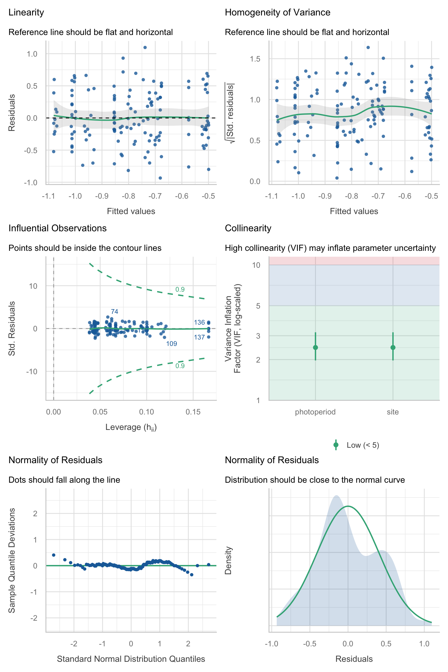
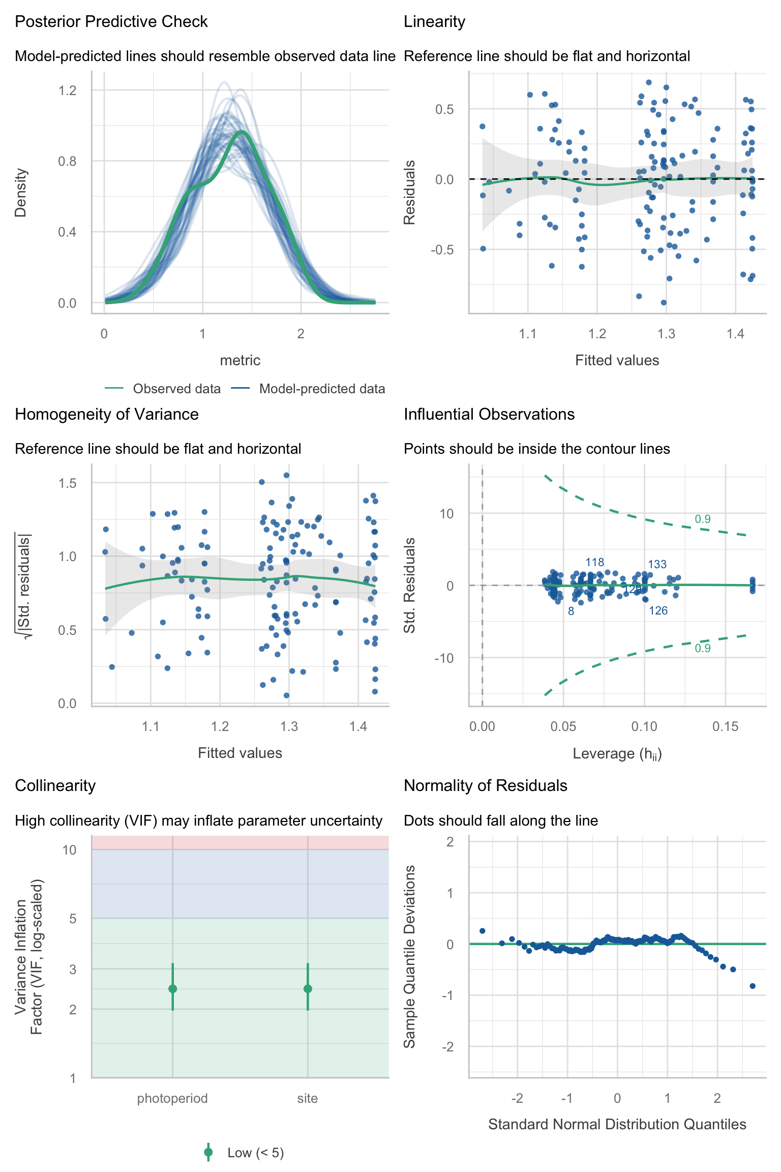
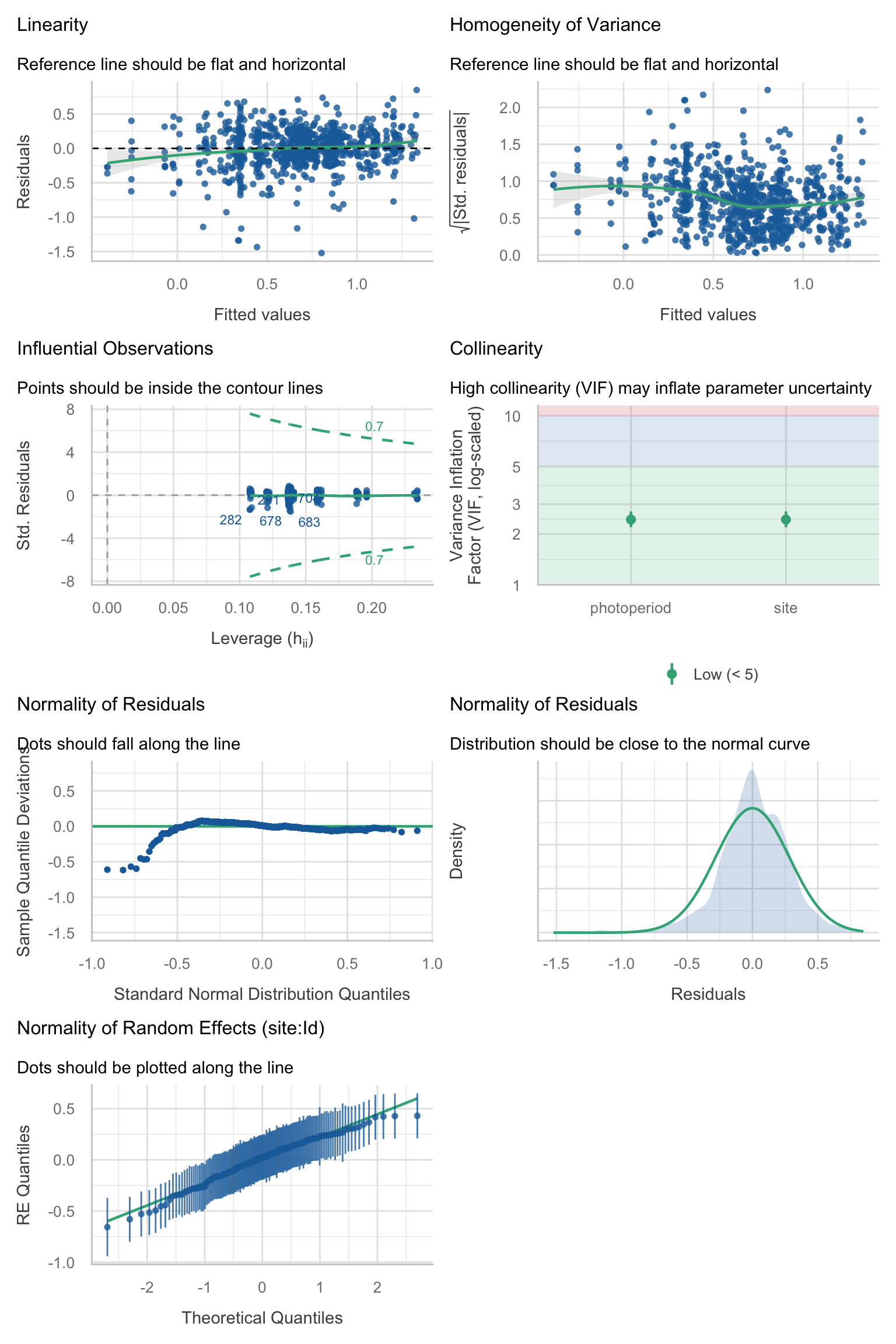
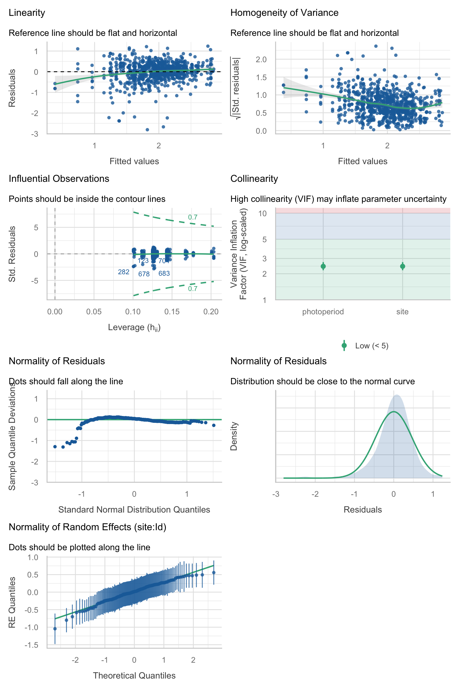
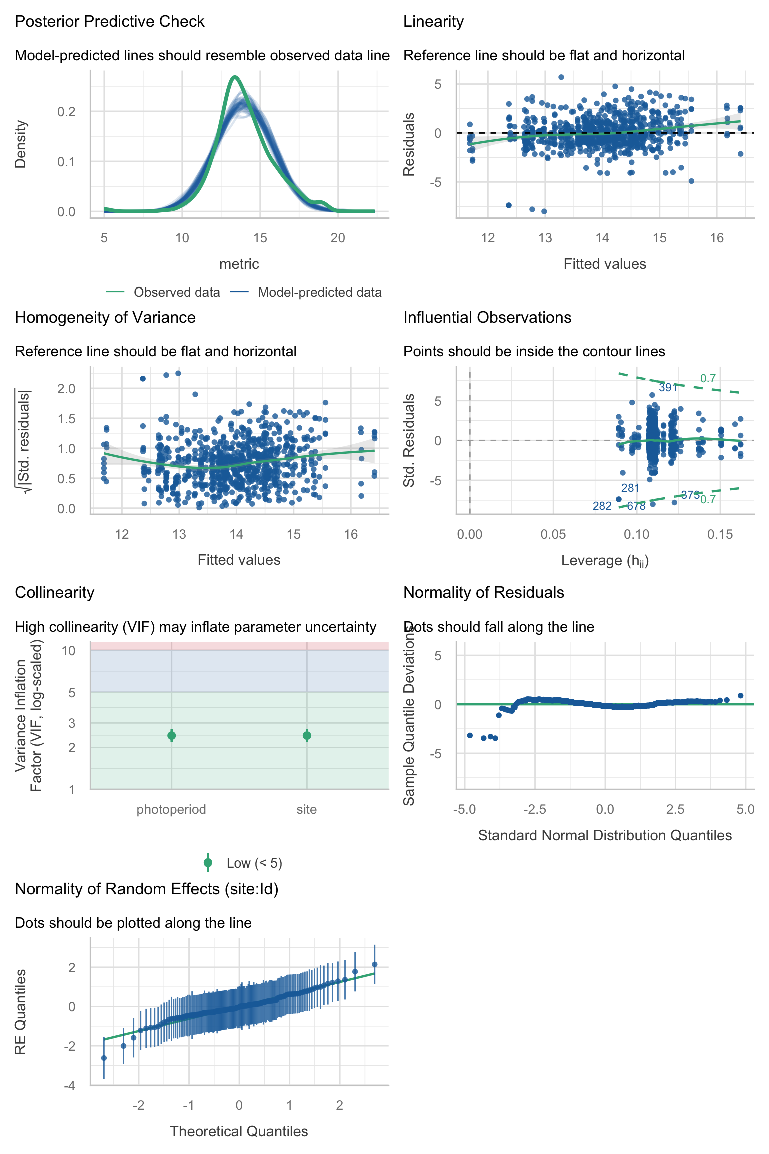
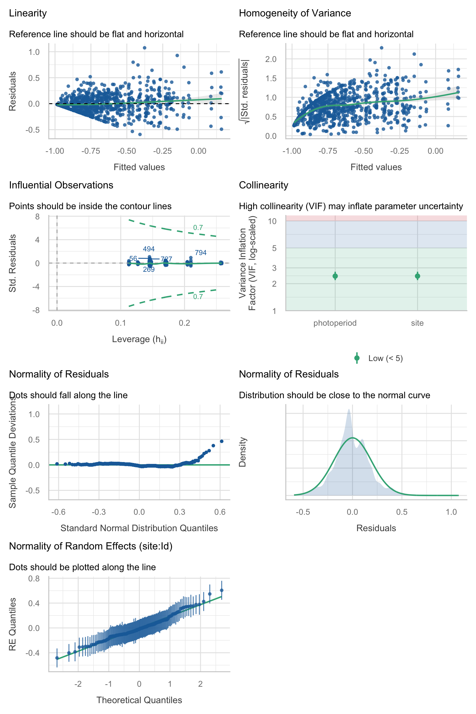
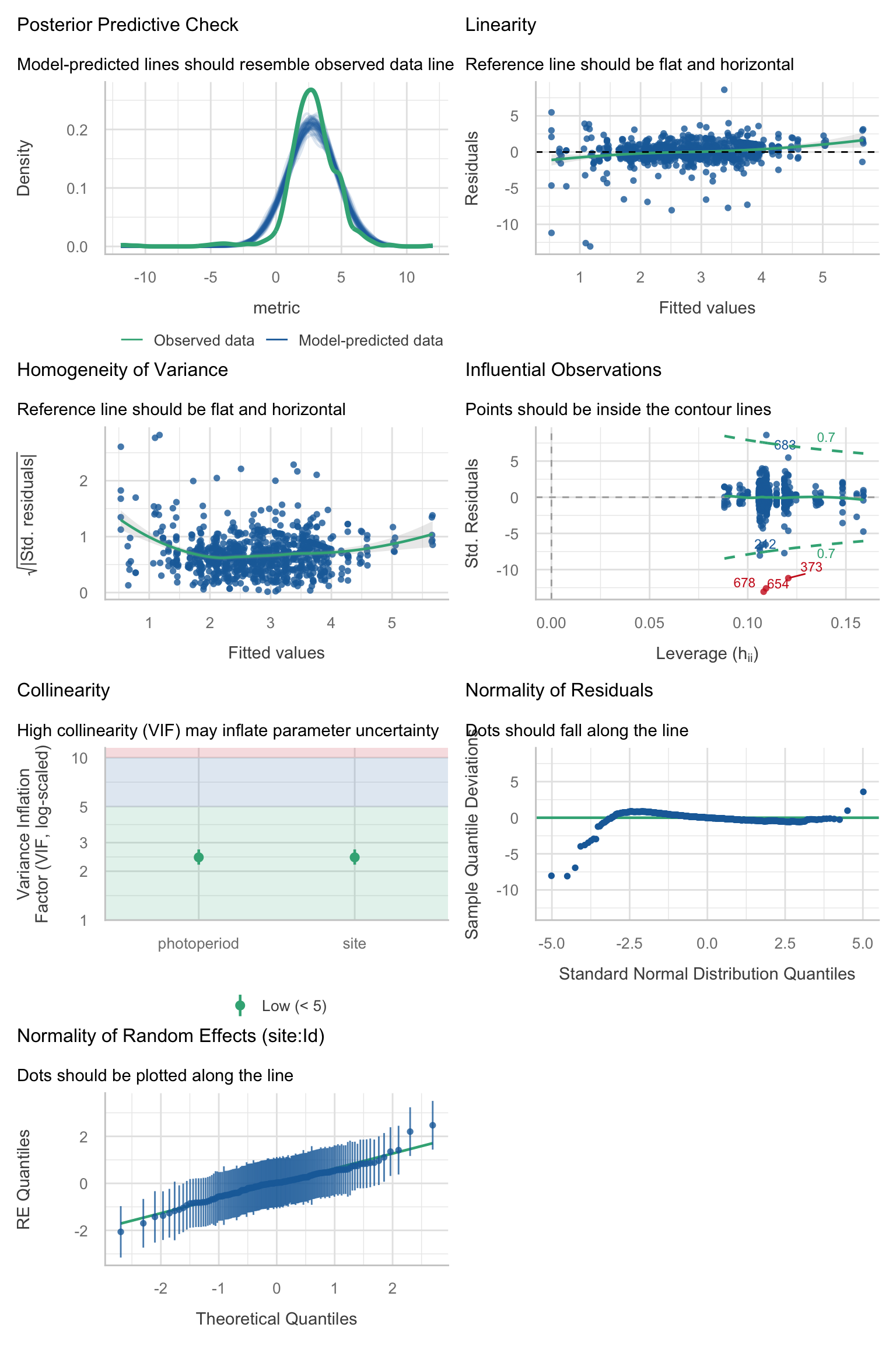
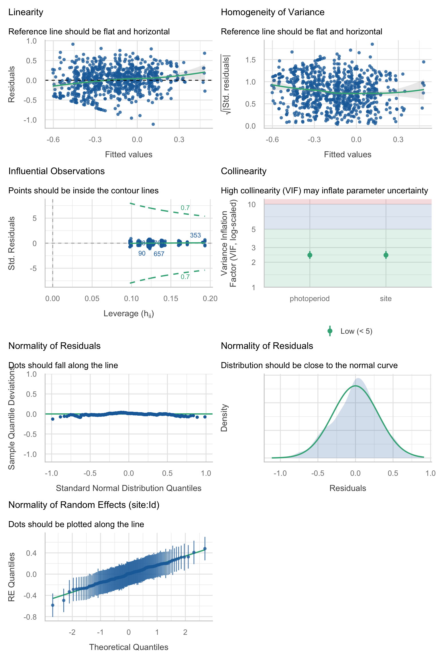
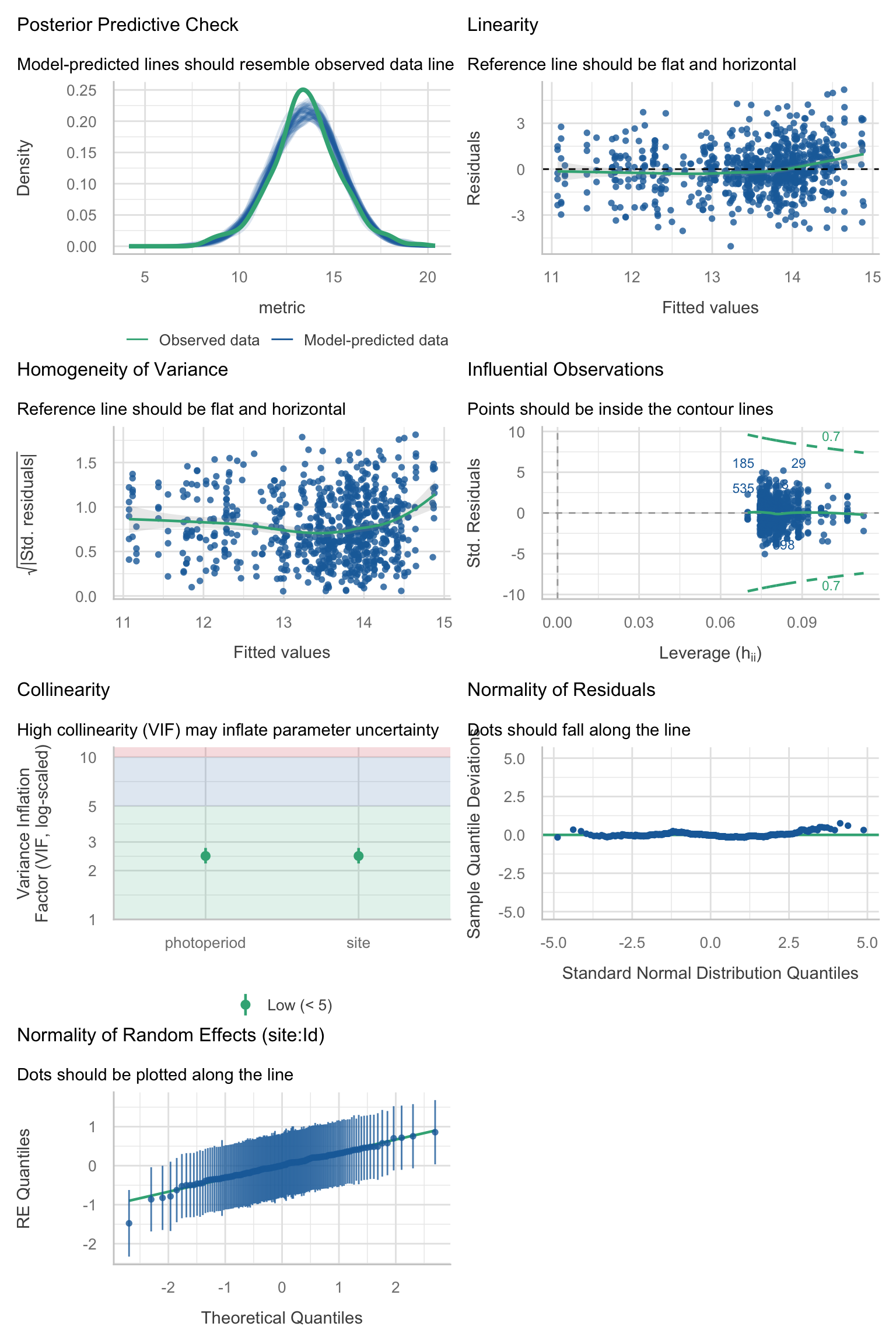
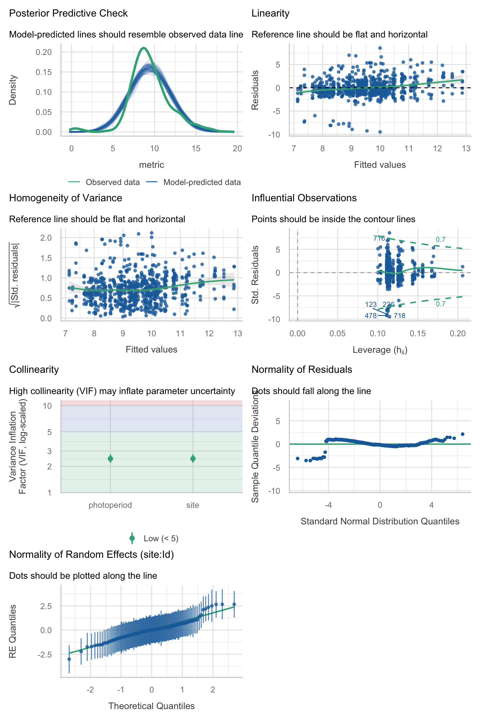
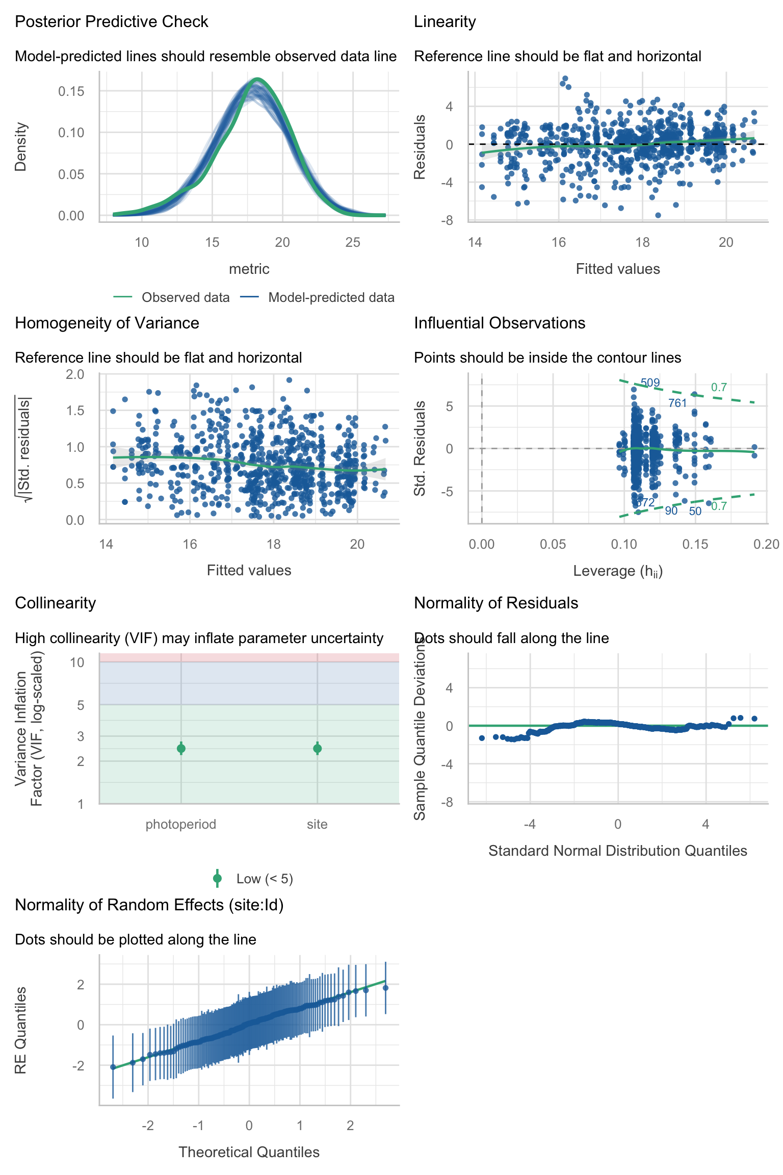
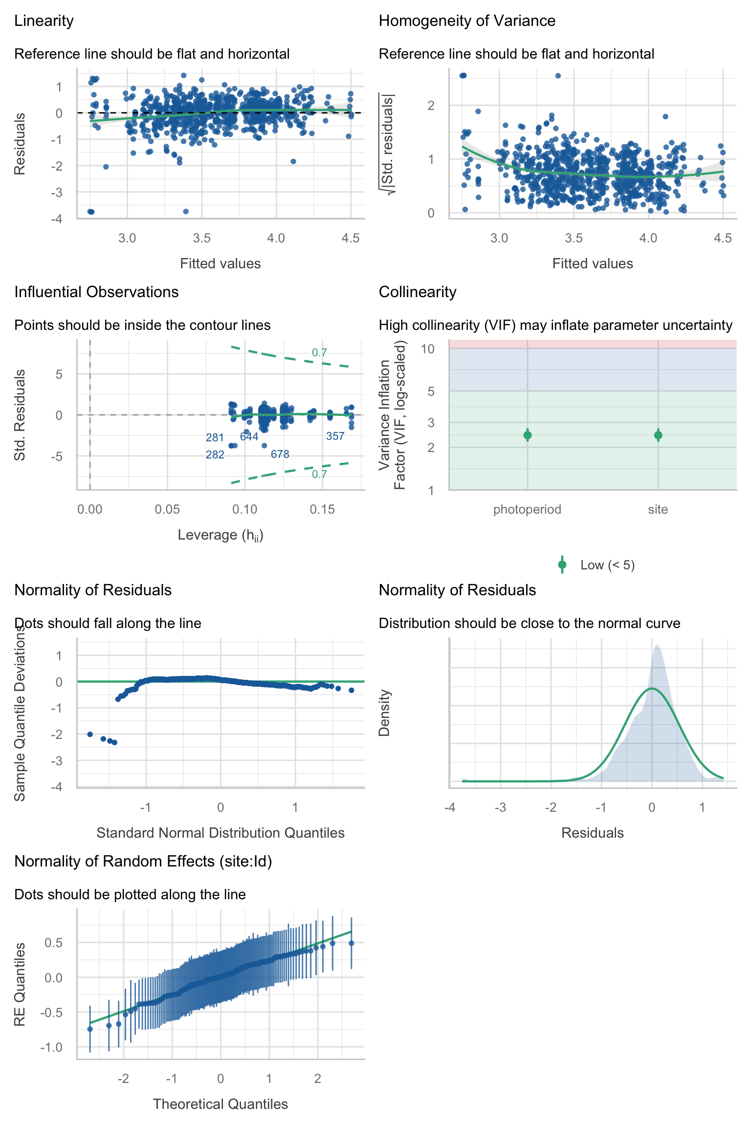
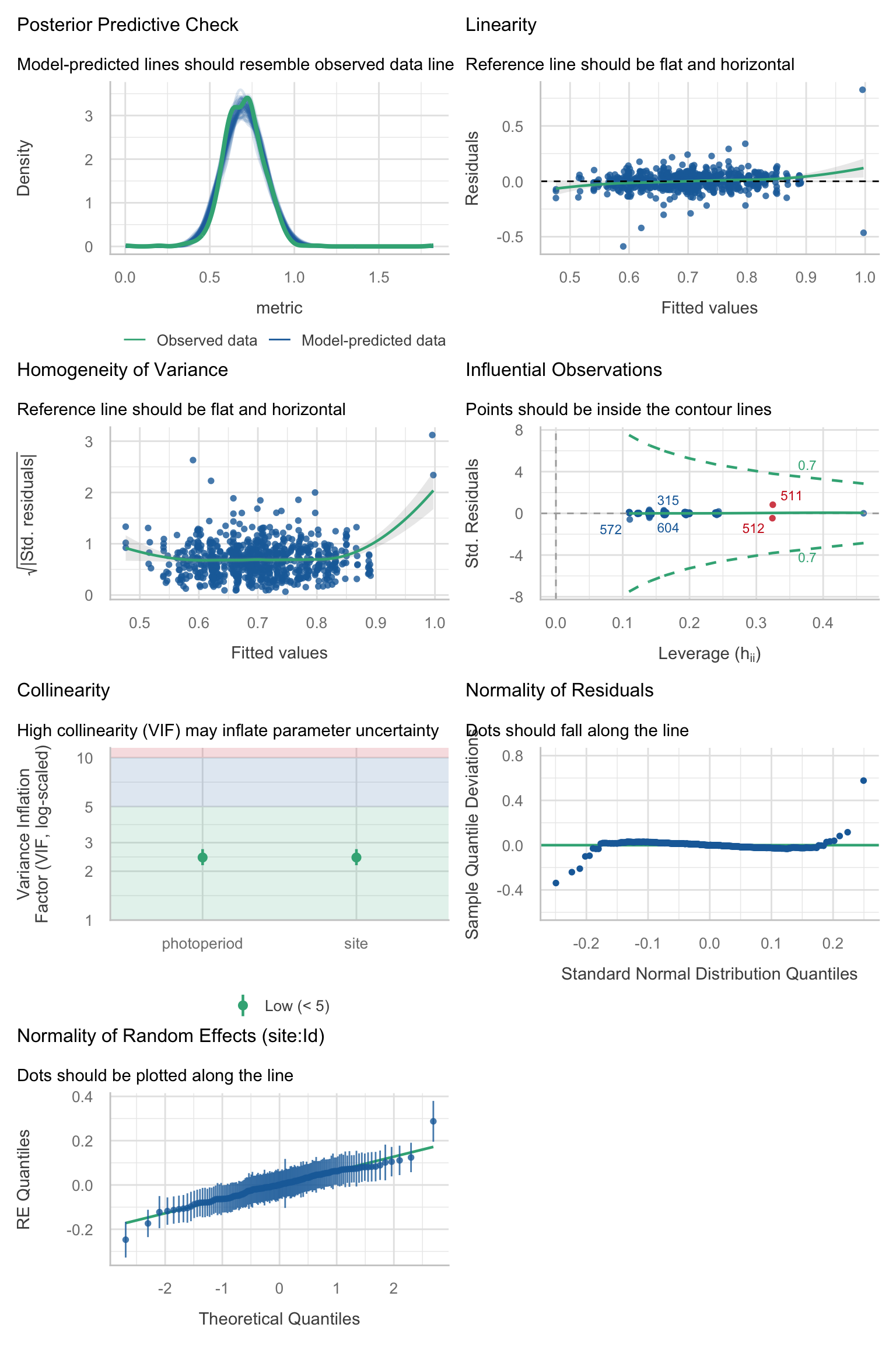
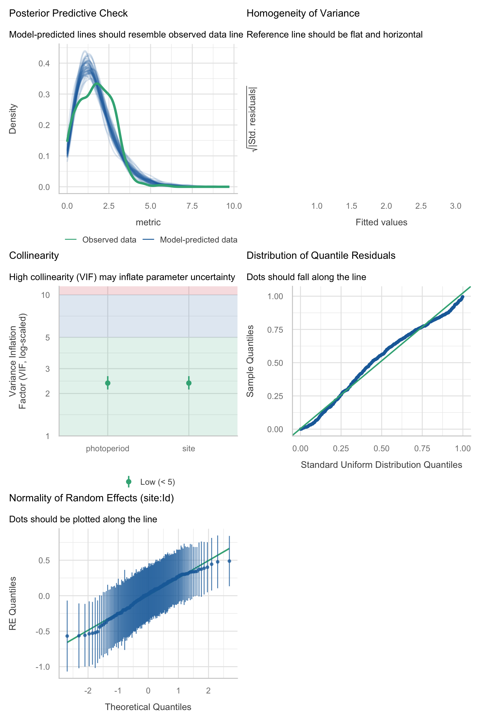
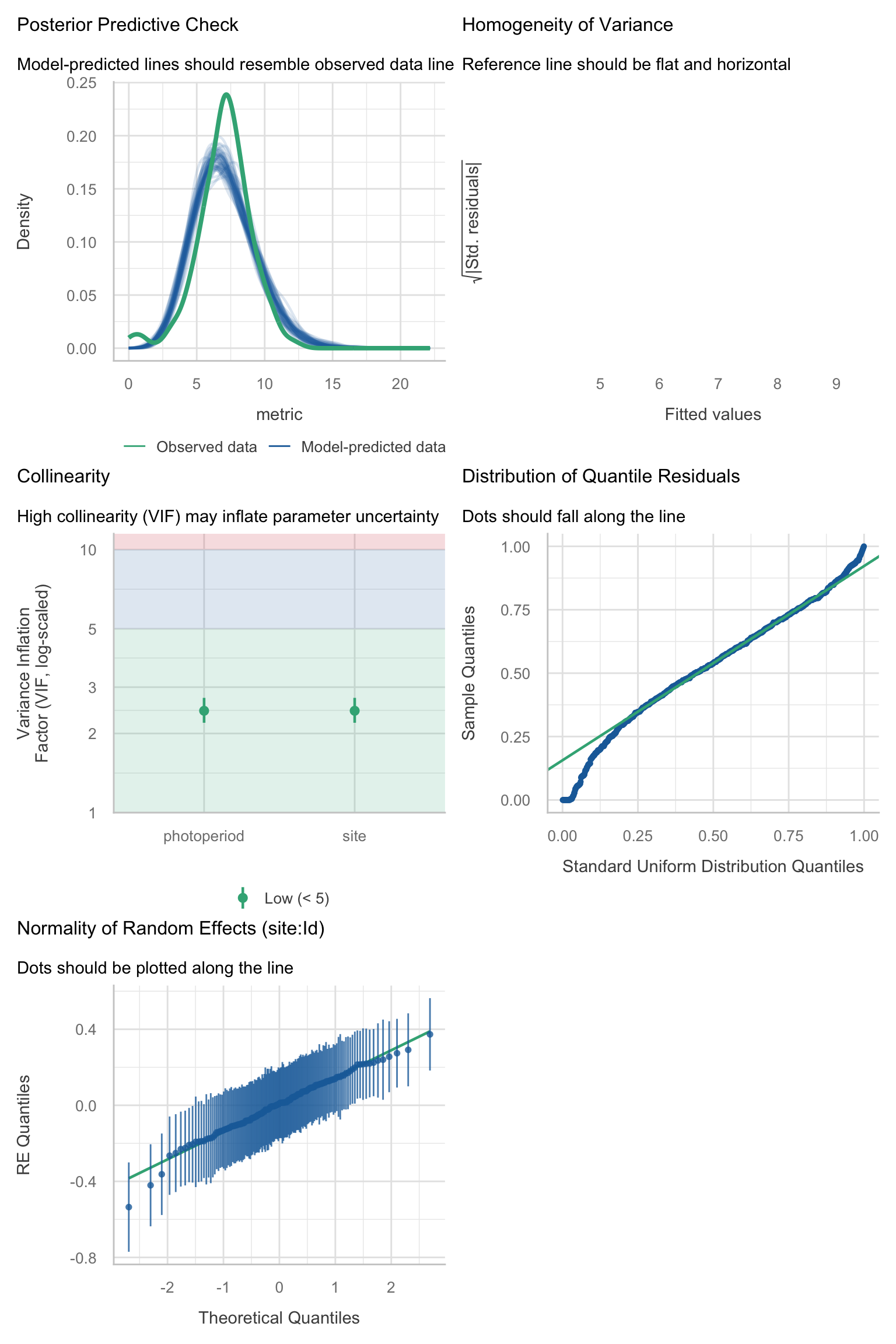
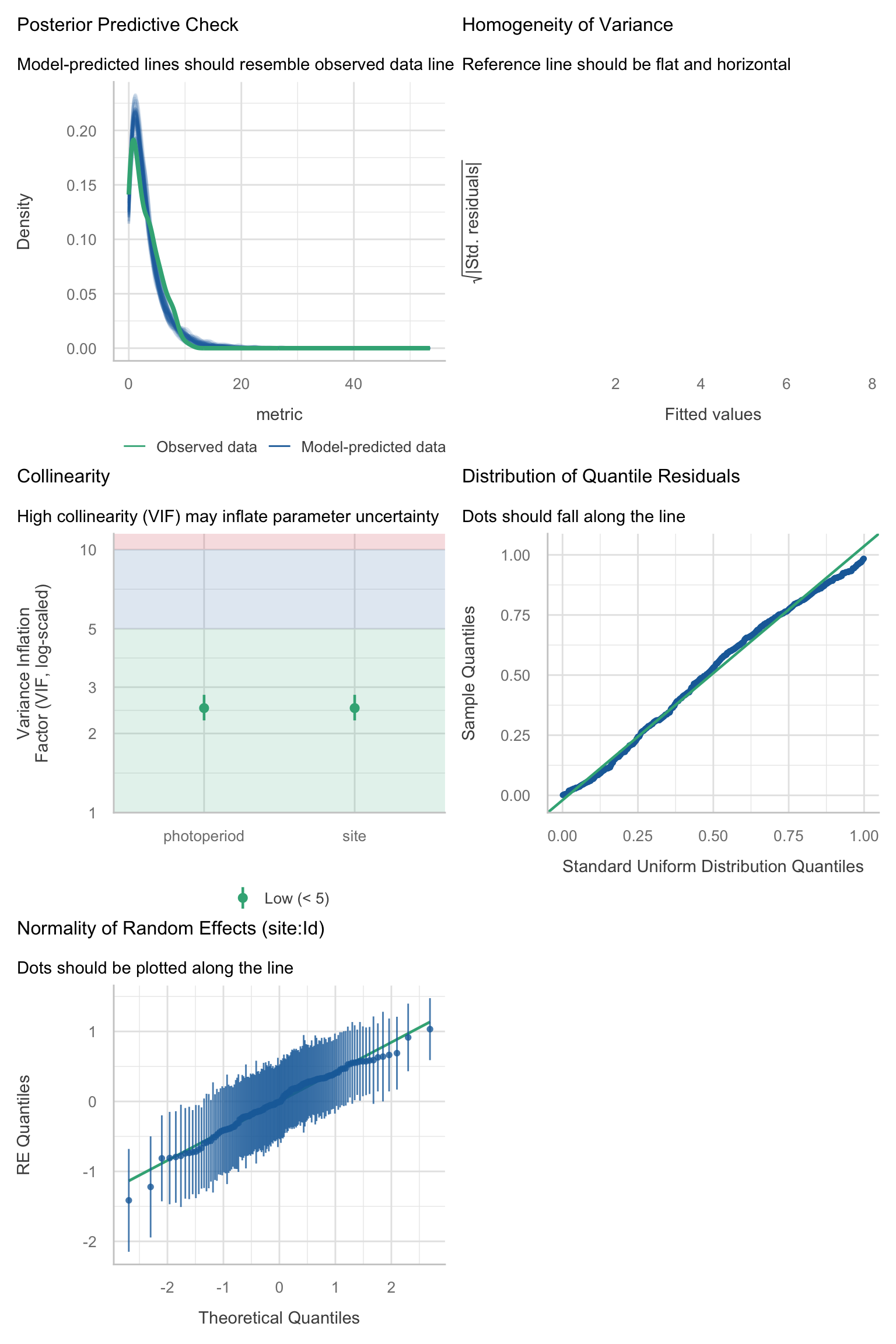
Model diagnostics overall look good to OK. Anomalies are found but deemed non-critical. Alternative error families, like the Tweedie distribution have been used as well. For Tweedie models, the homogeneity of variance does not show in the plots (duration metrics), but was checked interactively.

Model comparisons

In [10]:
Code cell - Model comparisons
metrics <- 
  metrics |> 
  mutate(
    H1_1_comp = map2(H1_0_model, H1_1_model, model_anova),
    H1_1_p = map2(H1_1_comp, engine, model_comp_p, n = H1_fdr_n) |> list_c(),
    H1_1_sig = H1_1_p <= sig.level,
    
    H1_lat_comp = map2(H1_0_model, H1_lat_model, model_anova),
    H1_lat_p = map2(H1_lat_comp, engine, model_comp_p, n = H1_fdr_n) |> list_c(),
    H1_lat_sig = H1_lat_p <= sig.level,
    
    H1_phot_comp = map2(H1_phot_model, H1_1_model, model_anova),
    H1_phot_p = map2(H1_phot_comp, engine, model_comp_p, n = H1_fdr_n) |> list_c(),
    H1_phot_sig = H1_phot_p <= sig.level,
    
    H1_rand_comp = map2(H1_0_model, H1_rand_model, model_anova),
    H1_rand_p = map2(H1_rand_comp, engine, model_comp_p, n = H1_fdr_n) |> list_c(),
    H1_rand_sig = H1_rand_p <= sig.level,
    
    AICs = pmap(list(H1_0_model, H1_1_model, H1_phot_model, H1_lat_model, 
                     H1_rand_model), model_AIC),
  
    summary = pmap(list(H1_1_sig, H1_0_model, H1_1_model), model_summary),
    summary_lat = pmap(list(H1_lat_sig, H1_0_model, H1_lat_model), model_summary),
    summary_rand = pmap(list(H1_rand_sig, H1_0_model, H1_rand_model),
                        model_summary),
  
    table = pmap(list(name, H1_1_p, summary, metric_type, 
                           response, family), model_table),
    table_lat = pmap(list(name, H1_lat_p, summary_lat, metric_type, 
                           response, family), model_table),
    table_lat = map(table_lat, \(x) if(is.null(x)) return() else x |>
                  mutate(across(any_of("lat"), \(x) x*10))),
    table = map2(table, H1_phot_sig, \(x,y) if(is.null(x)) return() else x |>
                  mutate(dAIC_photoperiod = ifelse(y, 0, -3))),
    table_rand = pmap(list(name, H1_rand_p, summary_rand, metric_type, 
                           response, family),model_table),
    table = pmap(list(table, table_lat, AICs, "lat", "H1_1", "H1_lat"),
                 H1_combining_tables),
    table = pmap(list(table, table_rand, AICs, "SD Site", "H1_1", "H1_rand"),
                 H1_combining_tables),
    )
refitting model(s) with ML (instead of REML)

R^2

In [11]:
Code cell - calculate R^2
R2_table <- 
  metrics |> 
  filter_out(is.na(response)) |> 
  mutate(
    name = name,
    metric_type = metric_type,
    H1_1_r2 = pmap(list(H1_1_model, data, family, response), r2_helper), 
    H1_0_r2 = pmap(list(H1_0_model, data, family, response), r2_helper), 
    H1_phot_r2 = pmap(list(H1_phot_model, data, family, response), r2_helper), 
    H1_lat_r2 = pmap(list(H1_lat_model, data, family, response), r2_helper), 
    H1_phot_sig = H1_phot_sig,
    H1_lat_sig = H1_lat_sig,
    H1_1_sig = H1_1_sig,
    .keep = "none"
  )
In [12]:
Code cell - choose relevant R^2
R2_table <- 
  R2_table |> 
  rowwise() |> 
  mutate(
    name = name,
    metric_type = metric_type,
    marginal_r2 = ifelse(H1_1_sig, H1_1_r2$R2_marginal, H1_0_r2$R2_marginal),
    conditional_r2 = ifelse(H1_1_sig, H1_0_r2$R2_conditional, H1_0_r2$R2_conditional),
    site_r2 = ifelse(H1_1_sig, H1_1_r2$R2_marginal - H1_0_r2$R2_marginal, NA),
    phot_r2 = ifelse(H1_phot_sig, H1_1_r2$R2_marginal - H1_phot_r2$R2_marginal, NA),
    rand_r2 = ifelse(H1_1_sig, H1_1_r2$R2_conditional - H1_1_r2$R2_marginal, #
                     H1_0_r2$R2_conditional - H1_0_r2$R2_marginal),
    rand_r2 = ifelse(rand_r2 == 0, NA, rand_r2),
    lat_r2 = ifelse(H1_lat_sig, H1_lat_r2$R2_marginal - H1_0_r2$R2_marginal, NA),
    .keep = "none"
  ) |> 
  mutate(across(c(marginal_r2, conditional_r2), 
                \(x) ifelse(metric_type == "dynamics", NA, x)
                ),
             phot_r2 = ifelse(is.na(site_r2) & !is.na(conditional_r2), marginal_r2, phot_r2)
         )

Results

In [13]:
Code cell - Table H1
H1_tab <- H1_table(metrics, H1_fdr_n) |> cols_width(Plot ~ px(200))
H1_tab
Picking joint bandwidth of 0.178
Picking joint bandwidth of 0.161
Warning: Removed 56 rows containing non-finite outside the scale range
(`stat_density_ridges()`).
Picking joint bandwidth of 0.161
Warning: Removed 56 rows containing non-finite outside the scale range
(`stat_density_ridges()`).
Picking joint bandwidth of 0.108
Warning: Removed 31 rows containing non-finite outside the scale range
(`stat_density_ridges()`).
Picking joint bandwidth of 0.108
Warning: Removed 31 rows containing non-finite outside the scale range
(`stat_density_ridges()`).
Picking joint bandwidth of 0.0385
Warning: Removed 21 rows containing non-finite outside the scale range
(`stat_density_ridges()`).
Picking joint bandwidth of 0.0385
Warning: Removed 21 rows containing non-finite outside the scale range
(`stat_density_ridges()`).
Picking joint bandwidth of 0.134
Picking joint bandwidth of 0.0425
Picking joint bandwidth of 0.179
Picking joint bandwidth of 0.201
Picking joint bandwidth of 0.13
Picking joint bandwidth of 0.183
Picking joint bandwidth of 0.107
Picking joint bandwidth of 0.0374
Warning: Removed 86 rows containing non-finite outside the scale range
(`stat_density_ridges()`).
Picking joint bandwidth of 0.0374
Warning: Removed 86 rows containing non-finite outside the scale range
(`stat_density_ridges()`).
Picking joint bandwidth of 0.552
Picking joint bandwidth of 0.5
Picking joint bandwidth of 0.676
Warning: Removed 33 rows containing non-finite outside the scale range
(`stat_density_ridges()`).
Picking joint bandwidth of 0.676
Warning: Removed 33 rows containing non-finite outside the scale range
(`stat_density_ridges()`).
Picking joint bandwidth of 0.769
Warning: Removed 33 rows containing non-finite outside the scale range
(`stat_density_ridges()`).
Picking joint bandwidth of 0.769
Warning: Removed 33 rows containing non-finite outside the scale range
(`stat_density_ridges()`).
Picking joint bandwidth of 0.578
Warning: Removed 33 rows containing non-finite outside the scale range
(`stat_density_ridges()`).
Picking joint bandwidth of 0.578
Warning: Removed 33 rows containing non-finite outside the scale range
(`stat_density_ridges()`).
Code cell - Table H1
gtsave(H1_tab, "tables/H1.png", vwidth = 1700)
Picking joint bandwidth of 0.178
Picking joint bandwidth of 0.161
Warning: Removed 56 rows containing non-finite outside the scale range
(`stat_density_ridges()`).
Picking joint bandwidth of 0.161
Warning: Removed 56 rows containing non-finite outside the scale range
(`stat_density_ridges()`).
Picking joint bandwidth of 0.108
Warning: Removed 31 rows containing non-finite outside the scale range
(`stat_density_ridges()`).
Picking joint bandwidth of 0.108
Warning: Removed 31 rows containing non-finite outside the scale range
(`stat_density_ridges()`).
Picking joint bandwidth of 0.0385
Warning: Removed 21 rows containing non-finite outside the scale range
(`stat_density_ridges()`).
Picking joint bandwidth of 0.0385
Warning: Removed 21 rows containing non-finite outside the scale range
(`stat_density_ridges()`).
Picking joint bandwidth of 0.134
Picking joint bandwidth of 0.0425
Picking joint bandwidth of 0.179
Picking joint bandwidth of 0.201
Picking joint bandwidth of 0.13
Picking joint bandwidth of 0.183
Picking joint bandwidth of 0.107
Picking joint bandwidth of 0.0374
Warning: Removed 86 rows containing non-finite outside the scale range
(`stat_density_ridges()`).
Picking joint bandwidth of 0.0374
Warning: Removed 86 rows containing non-finite outside the scale range
(`stat_density_ridges()`).
Picking joint bandwidth of 0.552
Picking joint bandwidth of 0.5
Picking joint bandwidth of 0.676
Warning: Removed 33 rows containing non-finite outside the scale range
(`stat_density_ridges()`).
Picking joint bandwidth of 0.676
Warning: Removed 33 rows containing non-finite outside the scale range
(`stat_density_ridges()`).
Picking joint bandwidth of 0.769
Warning: Removed 33 rows containing non-finite outside the scale range
(`stat_density_ridges()`).
Picking joint bandwidth of 0.769
Warning: Removed 33 rows containing non-finite outside the scale range
(`stat_density_ridges()`).
Picking joint bandwidth of 0.578
Warning: Removed 33 rows containing non-finite outside the scale range
(`stat_density_ridges()`).
Picking joint bandwidth of 0.578
Warning: Removed 33 rows containing non-finite outside the scale range
(`stat_density_ridges()`).
file:////var/folders/9p/326_k3kx43qbn_cyl1rqfhb00000gn/T//Rtmp81Ms5S/file1488eb3c072a.html screenshot completed
Code cell - Table H1
save(metrics, file = "data/H1_results.RData")
In [14]:
Model results for Hypothesis 1
Hypothesis: There is a significant difference in personal light-exposure metrics across sites, even after accounting for latitude and photoperiod.
Coefs are2 p-value3 Intercept
Site intercept (±coefficients)1
Photoperiod4,5 SD Participant SD Residual6
Comparative models
Distribution8
Borås (SE) Delft (NL) Dortmund (DE) Tübingen (DE) Munich (DE) Madrid (ES) Izmir (TR) San José (CR) Kumasi (GH) Latitude4,7 SD Site4,7
Duration
Duration above 1000 multiplied >0.9 5m 43s 1.17 1.84
Duration above 250 wake multiplied 0.062 38m 26s 1.10 1.77
Duration below 10 pre-Sleep multiplied >0.9 2h 31m 0.97 1.40
Duration below 1 sleep multiplied >0.9 8h 57m 0.98 1.20
Period above 250 multiplied >0.9 10m 27s 1.10 1.63 2.12
Dynamics9
Interdaily stability logit scale >0.9 −0.15 −0.05
Intradaily variability additive >0.9 1.33 0.00
Exposure History
Dose multiplied >0.9 356 1.19 2 4
Level
Mean multiplied 0.007 0.41 1.13 1.05 1.00 1.61 1.08 1.13 1.47 1.25 0.54 1.18 1.82 2.02 1.15 1.32
Brightest 10h mean multiplied 0.040 3.94 1.54 1.14 1.00 1.54 0.76 1.50 1.14 1.06 0.43 1.25 2.22 3.17 1.24
Darkest 10h mean multiplied <0.001 0.06 0.88 1.03 1.00 1.61 1.60 0.90 1.78 1.71 0.81 1.09 1.63 1.60 1.34
Spectrum
MDER additive 0.3 0.48 0.02 0.08 0.08
Timing
Brightest 10h midpoint additive 0.002 13.47 −48m 25s −2m 5s 0s −2m 50s 26m 22s 25m 44s 21m 10s −1h 20m −56m 2s 2m 32s 50m 28s 1h 34m 12m 8s 32m 16s
Darkest 10h midpoint additive 0.010 4.88 −32m 38s −17m 11s 0s 3m 26s 48m 27s −2m 22s 25m 7s −44m 36s −1h 6m −8m 40s 51m 11s 1h 38m
First timing above 250 additive 0.4 11.39 −8m 18s 1h 14m 2h 6m
Last timing above 250 additive <0.001 13.18 10m 19s 9m 56s 0s −16m 38s 33m 58s 1h 13m 44m 12s −2h 15m −1h 50m 19m 50s 1h 4m 2h 2m 28m 29s 1h 3m
Mean timing above 250 additive <0.001 11.81 −28m 17s 17m 41s 0s 1m 17s 11m 26s 39m 29s 39m 14s −2h 7m −1h 18m 7m 27s 33m 11s 1h 34m 21m 17s 52m 9s
1 Sites have only entries if the (adjusted) p-value is significant, otherwise the results for the null-model are shown. Entries show the site intercept, with the site-specific coefficient below in brackets (relative to the reference level).
2 multiplied: coefficients are multiplicative. This comes from the fact that the models were calculated on a log scale and backtransformed in the table. The Intercept can be read as linear scale, with coefficients being multiplied with the intercept. additive: All values are on the linear scale and no transformation is necessary. logit scale: data were modelled on the logit scale. Coefficients can be added to the intercept, but have to be transformed with the logistic function.
3 p-values are adjusted for multiple comparisons using the false-discovery-rate for n= 17 comparisons
4 Photoperiod: coefficient per 1-hour change in photoperiod. Latitude: coefficient per 10° change in latitude. SD Site: random effect standard deviation for site.
5 If the coefficient is greyed out it means it is not significant in a model base minus photoperiod.
6 Models with a tweedie error distribution do not return a residual standard deviation, as a dispersion parameter is estimated instead during modeling.
7 These coefficients (Latitude) and random effects (SD Site) come from two respective separate models that did not contain a fixed effect of site. If the random site or fixed latitude effect is significant, a value is presented. If AIC indicates a significant improvement over the base model (site as fixed effect), it is shown in bold. If the base model is significantly stronger, however, values are shown in grey.
8 When coefficients are multiplicative (see column), then the scaling is on a log 10 base, with an offset of +0.1. Red horizontal lines indicate the median of a site.
9 Dynamics-based metrics are calculated per participant and thus are using linear/generalized models instead of the mixed-model framework

Interpretation

@tbl-H1 shows a comprehensive overview of the main inference results. When site is significant, site coefficients are with reference to the BAUA site.

As way of a high-level summary:

  • Timing-based metrics show a significant site-specific effect that is neither dependent on photoperiod, nor latitude
  • While level-based metrics show a significant site-specific effect, it can be drawn back to photoperiod and latitude for daytime metrics (but not for nighttime)
  • Duration-based metrics are photoperiod-dependent, but not site specific, same as exposure history and spectrum - these metrics are rather more dependent on inter- and intraindividual differences of participants
  • In general, interindividual differences highly relevant and trump site specific factors, although usually not as large as intraindividual differences
  • None of the above means that individual sites can not be significantly different from the group or another site. But rather that the variance across all nine sites is or is not sufficiently large.
Timing and level-based metrics prove site specific
  • Both timing and level-based metrics show site specificity, even when controlled for photoperiod
  • The First timing above 250 lx melanopic EDI (timing) is the only exception, with neither site nor photoperiod-specific influence
  • Neither duration, dynamics, exposure history, nor spectrum-based metrics show site specificity
Level-based
  • For the overall daily Mean, slight increases over BAUA (100%) are THUAS (+5%), TUM (+6%), FUSPCEU(+13%), RISE (+14%), and UCR(+25%). Quite higher are IZTECH (+47%) and MPI(+62%). Quite darker is KNUST (-46%)
  • For the Brightest 10h mean, slight increases over BAUA (100%) are UCR(+7%), THUAS (+14%) and IZTECH(+15%). Quite brighter are FUSPCEU(+50%), MPI(+54%), and RISE(+55%). Darker are TUM (-25%) and KNUST(-46%)
  • For the Darkest 10h mean, slight increases over BAUA (100%) are THUAS(+3%). Quite brighter are MPI(+61%), TUM(+64%), UCR(+71%), and IZTECH(+78%). Darker are FUSPCEU(-10%), RISE(-12%), and KNUST()
Timing-based
  • Values are rounded to full minutes
  • For the Brightest 10h midpoint, we see shifts to later timing relative to BAUA from IZTECH(+20min), FUSPCEU(+26min), and TUM(+31min). Sites with earlier timing are THUAS(-2min), MPI(-2min), RISE(-45min), KNUST(-57min), and UCR(-1h 19min)
  • For the Darkest 10h midpoint, we see shifts to later timing relative to BAUA from MPI(+4min), IZTECH(+25min), and TUM(+51min). Sites with earlier timing are FUSPCEU(-2min), THUAS(-19min), RISE(-33min), UCR(-45min), and KNUST(-1h 7min)
  • For the Last timing above 250lx melanopic EDI, we see shifts to later timing relative to BAUA from RISE(+2min), THUAS(+7min), TUM(+26min), IZTECH(+44min), and FUSPCEU(+1h 5min). Sites with earlier timing are MPI(-17min), KNUST(-1h 56min), and UCR(-2h 12min)
  • For the Mean timing above 250lx melanopic EDI, we see shifts to later timing relative to BAUA from MPI(+0min), THUAS(+17min), TUM(+18min), IZTECH(+41min), and FUSPCEU(+41min). Sites with earlier timing are RISE(-28min), KNUST(-1h 19min), and UCR(-2h 4min).
Site effects are not random
  • With the exception of the Mean and the Darkest 10h mean (both based on logarithmic scaling), site coefficients are not randomly (normally) distributed, but rather show specific differences, even when controlled for photoperiod
  • for Mean, a random site factor translates to ± 32% for 1 standard deviation, and for the Darkest 10h mean ± 35% for 1 standard deviation
Latitude explains daytime levels better than site specifics coefficients
  • For the Mean and the Brightest 10h mean(both based on logarithmic scaling), latitude is a better predictor (based on ∆AIC) compared to the site (both controlled for photoperiod).
  • Per 10 degrees of latitude, the Mean increases by 15%, and the Brightest 10h mean by 24%
  • These coefficients are multiplicative, meaning that, e.g., a 30° latitude increase for Mean would not result in and \(3*15\%=45\%\) increase, but rather an increase of \(1.15^3=1.52=+52%\)
Photoperiod is highly relevant for duration, exposure history, level, and spectrum based metrics, but not for dynamics and timing based metrics
  • Photoperiod is significant for Dose (exposure history), MDER (spectrum), all level-based metrics, all duration-based metrics sans Duration below 1 lx melanopic EDI during sleep, and the Last timing above 250 lx melanopic EDI and Mean timing above 250 lx melanopic EDI (timing).
  • Photoperiod is not relevant for the Duration below 1 lx melanopic EDI during sleep (duration), dynamics-based metrics, and 3 out of 5 timing-based metrics (Brightest 10h midpoint, Darkest 10h midpoint, First timing above 250 lx melanopic EDI)
  • For duration-based metrics, every hour of photoperiod increases Duration above 1000 lx melanopic EDI (+17%), Duration above 250 lx melanopic EDI (+10%), and Period above 250 lx melanopic EDI (+10%). Every hour of photoperiod also decreases the Duration below 10 lx melanopic EDI during pre-sleep (-3%).
  • Dose is increased by +19% per hour of photoperiod
  • MDER is increased by 0.02 per hour of photoperiod
  • For level-based metrics, every hour of photoperiod increases the Mean (+18%), the Brightest 10h mean (+25%), the Darkest 10h mean (+9%)
  • For timing-based metrics, every hour of photoperiod shifts the Last timing above 250 lx melanopic EDI (+20 minutes) and the Mean timing above 250 lx melanopic EDI (+~8 minutes)
Interindividual and intraindividual differences outweigh site-specific differences
  • For both level and timing-based metrics interindividual differences (SD Participant) and intraindividual differences (SD Residual) outweigh most site-specific differences (i.e., coefficients)
  • However, the highest site-specific differences (hightest site coefficient minus lowest site coefficient) are in the range of intraindividual differences (1 standard deviation for SD Residual)
  • In most cases, intraindividual differences (SD Residual) outweigh interindividual differences (SD Participant). A notable exception is the Darkest 10h mean, where both are similar (SD Participant ±63% vs. SD Residual ±60%)

R2

In [15]:
Code cell - R^2 table
R2_tbl <- 
R2_table |> 
  mutate(metric_type = str_to_title(metric_type)) |> 
  arrange(metric_type, name) |> 
  group_by(metric_type) |> 
  gt(rowname_col = "name") |> 
  cols_add(Residual = 1 - conditional_r2) |> 
  fmt_percent(decimals = 0) |>
  sub_missing() |> 
  tab_header(md("**H1: Variance explained by the model parameters ($R^{2}$)**")) |> 
  fmt(name, 
      rows = name != "MDER",
      fns = \(x) x |> str_to_sentence() |> str_replace_all("_", " ")) |> 
  cols_move(rand_r2, after = lat_r2) |> 
  cols_move(marginal_r2, after = conditional_r2) |> 
  cols_label(
    conditional_r2 = "Model",
    rand_r2 = "Participants",
    marginal_r2 = "Fixed effects",
    site_r2 = "Site",
    phot_r2 = "Photoperiod",
    lat_r2 = "Latitude"
  ) |> 
  tab_spanner("Unique contribution", columns = c(site_r2, phot_r2, lat_r2)) |> 
  cols_width(
    name ~ px(230),
    phot_r2 ~ px(100),
    c(rand_r2, Residual) ~ px(90),
    everything() ~ px(70)) |> 
  grand_summary_rows(
    columns = where(is.numeric),
    fns = list(
      `Grand average` ~ mean(., na.rm = TRUE)
    ),
        side = "top",
    fmt = ~ fmt_percent(., decimals = 0)
  ) |> 
  tab_style(
    cell_text(align = "center"),
    list(cells_body(),
         cells_grand_summary(),
         cells_column_labels())
  ) |> 
    tab_style(
    cell_text(weight = "bold"),
    list(cells_column_labels(),
         cells_row_groups(),
         cells_grand_summary(),
         cells_stub_grand_summary())
  ) |> 
  tab_footnote(
    md("*Model*: conditional $R^2$, *Participants*: partial $R^2$ due to interindividual differences on a participant level, Fixed effects: marginal $R^2$ (all fixed effects combined, based on a model of $site + photoperiod$), *Site/Photoperiod/Latitude*: unique contribution of the given parameter relative to a model without it. *Residual*: proportion of residual variance (e.g., intraindividual differences)")
  )
In [16]:
Code
R2_tbl
H1: Variance explained by the model parameters (\(R^{2}\))
Model Fixed effects
Unique contribution
Participants Residual
Site Photoperiod Latitude
Grand average 40% 12% 10% 7% 5% 28% 60%
Duration
Duration above 1000 49% 17% 17% 33% 51%
Duration above 250 wake 51% 9% 9% 42% 49%
Duration below 10 pre-sleep 31% 2% 2% 29% 69%
Duration below 1 sleep 38% 3% 3% 35% 62%
Period above 250 35% 8% 8% 27% 65%
Dynamics
Interdaily stability
Intradaily variability
Exposure History
Dose 31% 9% 9% 22% 69%
Level
Mean 55% 24% 7% 8% 3% 32% 45%
Brightest 10h mean 43% 18% 6% 6% 4% 26% 57%
Darkest 10h mean 62% 23% 15% 3% 40% 38%
Spectrum
MDER 54% 13% 13% 41% 46%
Timing
Brightest 10h midpoint 27% 8% 8% 2% 20% 73%
Darkest 10h midpoint 27% 9% 6% 19% 73%
First timing above 250 28% 2% 2% 25% 72%
Last timing above 250 39% 23% 12% 5% 6% 17% 61%
Mean timing above 250 25% 17% 14% 1% 7% 9% 75%
Model: conditional \(R^2\), Participants: partial \(R^2\) due to interindividual differences on a participant level, Fixed effects: marginal \(R^2\) (all fixed effects combined, based on a model of \(site + photoperiod\)), Site/Photoperiod/Latitude: unique contribution of the given parameter relative to a model without it. Residual: proportion of residual variance (e.g., intraindividual differences)
Code
gtsave(R2_tbl, "tables/H1_R2_tbl.png")
file:////var/folders/9p/326_k3kx43qbn_cyl1rqfhb00000gn/T//Rtmp81Ms5S/file1488e78930394.html screenshot completed
  • Overall model fit varies widely (≈25–62%), with highest explanatory power for level-based metrics (e.g., darkest/mean light levels) and lowest for timing metrics.
  • Fixed effects explain a modest share (≈2–24%), indicating environmental factors (site, photoperiod, latitude) contribute but are not dominant drivers.
  • Individual (participant-level) differences account for a large portion of variance (≈20–42%), often exceeding fixed-effect contributions.
  • Site effects are generally stronger than photoperiod, particularly for level metrics, but both show overlapping (shared) explanatory power.
  • Latitude contributes only marginally where included, suggesting limited additional explanatory value beyond photoperiod.
  • Residual variance remains high across most metrics (≈38–75%), indicating substantial unexplained within-individual or day-to-day variability.

Model summaries

The following tabs show the model summaries for either

  • \(\text{Metric} \sim \text{Site} + \text{Photoperiod} + (1|\text{Site}:\text{Participant})\)

or

  • \(\text{Metric} \sim \text{Photoperiod} + (1|\text{Site}:\text{Participant})\)

depending on whether site is significant

Model summary

Characteristic Beta 95% CI p-value
photoperiod -0.05 -0.07, -0.02 <0.001
Abbreviation: CI = Confidence Interval

Model comparison

✖ Unable to identify the list of variables.

This is usually due to an error calling `stats::model.frame(x)`or `stats::model.matrix(x)`.
It could be the case if that type of model does not implement these methods.
Rarely, this error may occur if the model object was created within
a functional programming framework (e.g. using `lappy()`, `purrr::map()`, etc.).
Characteristic p-value
Model 1: qlogis(metric) ~ photoperiod
Model 2: qlogis(metric) ~ site + photoperiod 0.12

Model summary

Characteristic Beta 95% CI p-value
photoperiod 0.00 -0.03, 0.02 0.8
Abbreviation: CI = Confidence Interval

Model comparison

✖ Unable to identify the list of variables.

This is usually due to an error calling `stats::model.frame(x)`or `stats::model.matrix(x)`.
It could be the case if that type of model does not implement these methods.
Rarely, this error may occur if the model object was created within
a functional programming framework (e.g. using `lappy()`, `purrr::map()`, etc.).
Characteristic p-value
Model 1: metric ~ photoperiod
Model 2: metric ~ site + photoperiod 0.2

Model summary

Characteristic Beta 95% CI
site

    BAUA 0.00
    FUSPCEU 0.05 -0.18, 0.29
    IZTECH 0.17 -0.05, 0.38
    KNUST -0.27 -0.50, -0.04
    MPI 0.21 0.00, 0.42
    RISE 0.05 -0.15, 0.26
    THUAS 0.02 -0.19, 0.23
    TUM 0.03 -0.19, 0.26
    UCR 0.10 -0.19, 0.38
photoperiod 0.07 0.05, 0.10
Abbreviation: CI = Confidence Interval

Model comparison

✖ Unable to identify the list of variables.

This is usually due to an error calling `stats::model.frame(x)`or `stats::model.matrix(x)`.
It could be the case if that type of model does not implement these methods.
Rarely, this error may occur if the model object was created within
a functional programming framework (e.g. using `lappy()`, `purrr::map()`, etc.).
Characteristic p-value
model1: log_zero_inflated(metric) ~ photoperiod + (1 | site:Id)
model2: log_zero_inflated(metric) ~ site + photoperiod + (1 | site:Id) <0.001

Model summary

Characteristic Beta 95% CI
site

    BAUA 0.00
    FUSPCEU 0.18 -0.15, 0.51
    IZTECH 0.06 -0.24, 0.36
    KNUST -0.37 -0.69, -0.05
    MPI 0.19 -0.10, 0.48
    RISE 0.19 -0.10, 0.48
    THUAS 0.06 -0.24, 0.35
    TUM -0.12 -0.43, 0.19
    UCR 0.03 -0.37, 0.43
photoperiod 0.10 0.06, 0.13
Abbreviation: CI = Confidence Interval

Model comparison

✖ Unable to identify the list of variables.

This is usually due to an error calling `stats::model.frame(x)`or `stats::model.matrix(x)`.
It could be the case if that type of model does not implement these methods.
Rarely, this error may occur if the model object was created within
a functional programming framework (e.g. using `lappy()`, `purrr::map()`, etc.).
Characteristic p-value
model1: log_zero_inflated(metric) ~ photoperiod + (1 | site:Id)
model2: log_zero_inflated(metric) ~ site + photoperiod + (1 | site:Id) 0.002

Model summary

Characteristic Beta 95% CI
site

    BAUA 0.00
    FUSPCEU 0.43 -0.45, 1.3
    IZTECH 0.35 -0.45, 1.2
    KNUST -0.93 -1.8, -0.08
    MPI -0.05 -0.82, 0.72
    RISE -0.81 -1.6, -0.05
    THUAS -0.03 -0.81, 0.74
    TUM 0.44 -0.38, 1.3
    UCR -1.3 -2.4, -0.27
photoperiod 0.04 -0.06, 0.14
Abbreviation: CI = Confidence Interval

Model comparison

✖ Unable to identify the list of variables.

This is usually due to an error calling `stats::model.frame(x)`or `stats::model.matrix(x)`.
It could be the case if that type of model does not implement these methods.
Rarely, this error may occur if the model object was created within
a functional programming framework (e.g. using `lappy()`, `purrr::map()`, etc.).
Characteristic p-value
model1: metric ~ photoperiod + (1 | site:Id)
model2: metric ~ site + photoperiod + (1 | site:Id) <0.001

Model summary

Characteristic Beta 95% CI
site

    BAUA 0.00
    FUSPCEU -0.04 -0.23, 0.14
    IZTECH 0.25 0.08, 0.42
    KNUST -0.09 -0.28, 0.09
    MPI 0.21 0.04, 0.37
    RISE -0.05 -0.22, 0.11
    THUAS 0.01 -0.15, 0.18
    TUM 0.20 0.03, 0.38
    UCR 0.23 0.01, 0.46
photoperiod 0.04 0.01, 0.06
Abbreviation: CI = Confidence Interval

Model comparison

✖ Unable to identify the list of variables.

This is usually due to an error calling `stats::model.frame(x)`or `stats::model.matrix(x)`.
It could be the case if that type of model does not implement these methods.
Rarely, this error may occur if the model object was created within
a functional programming framework (e.g. using `lappy()`, `purrr::map()`, etc.).
Characteristic p-value
model1: log_zero_inflated(metric) ~ photoperiod + (1 | site:Id)
model2: log_zero_inflated(metric) ~ site + photoperiod + (1 | site:Id) <0.001

Model summary

Characteristic Beta 95% CI
site

    BAUA 0.00
    FUSPCEU -0.04 -0.94, 0.86
    IZTECH 0.42 -0.40, 1.2
    KNUST -1.1 -2.0, -0.24
    MPI 0.06 -0.73, 0.85
    RISE -0.54 -1.3, 0.23
    THUAS -0.29 -1.1, 0.51
    TUM 0.81 -0.03, 1.6
    UCR -0.74 -1.8, 0.35
photoperiod -0.14 -0.25, -0.04
Abbreviation: CI = Confidence Interval

Model comparison

✖ Unable to identify the list of variables.

This is usually due to an error calling `stats::model.frame(x)`or `stats::model.matrix(x)`.
It could be the case if that type of model does not implement these methods.
Rarely, this error may occur if the model object was created within
a functional programming framework (e.g. using `lappy()`, `purrr::map()`, etc.).
Characteristic p-value
model1: metric ~ photoperiod + (1 | site:Id)
model2: metric ~ site + photoperiod + (1 | site:Id) <0.001

Model summary

Warning: the 'nobars' function has moved to the reformulas package. Please update your imports, or ask an upstream package maintainer to do so.
This warning is displayed once per session.
ℹ Multinomial models, multi-component models and other groups models have a
  different underlying structure than the models gtsummary was designed for.
• Functions designed to work with `tbl_regression()` objects may yield
  unexpected results.
ℹ Suppress this message with `?suppressMessages()`.
Characteristic Beta 95% CI p-value
cond
photoperiod 0.16 0.12, 0.21 <0.001
Abbreviation: CI = Confidence Interval

Model comparison

✖ Unable to identify the list of variables.

This is usually due to an error calling `stats::model.frame(x)`or `stats::model.matrix(x)`.
It could be the case if that type of model does not implement these methods.
Rarely, this error may occur if the model object was created within
a functional programming framework (e.g. using `lappy()`, `purrr::map()`, etc.).
Characteristic p-value
model1: metric ~ photoperiod + (1 | site:Id), zi=~0, disp=~1
model2: metric ~ site + photoperiod + (1 | site:Id), zi=~0, disp=~1 0.058

Model summary

Characteristic Beta 95% CI
photoperiod 0.04 0.03, 0.06
Abbreviation: CI = Confidence Interval

Model comparison

✖ Unable to identify the list of variables.

This is usually due to an error calling `stats::model.frame(x)`or `stats::model.matrix(x)`.
It could be the case if that type of model does not implement these methods.
Rarely, this error may occur if the model object was created within
a functional programming framework (e.g. using `lappy()`, `purrr::map()`, etc.).
Characteristic p-value
model1: log_zero_inflated(metric) ~ photoperiod + (1 | site:Id)
model2: log_zero_inflated(metric) ~ site + photoperiod + (1 | site:Id) 0.3

Model summary

Characteristic Beta 95% CI
site

    BAUA 0.00
    FUSPCEU 0.66 -0.06, 1.4
    IZTECH 0.65 0.00, 1.3
    KNUST -1.3 -2.0, -0.60
    MPI 0.02 -0.61, 0.66
    RISE -0.47 -1.1, 0.14
    THUAS 0.29 -0.34, 0.93
    TUM 0.19 -0.48, 0.86
    UCR -2.1 -3.0, -1.3
photoperiod 0.12 0.04, 0.21
Abbreviation: CI = Confidence Interval

Model comparison

✖ Unable to identify the list of variables.

This is usually due to an error calling `stats::model.frame(x)`or `stats::model.matrix(x)`.
It could be the case if that type of model does not implement these methods.
Rarely, this error may occur if the model object was created within
a functional programming framework (e.g. using `lappy()`, `purrr::map()`, etc.).
Characteristic p-value
model1: metric ~ photoperiod + (1 | site:Id)
model2: metric ~ site + photoperiod + (1 | site:Id) <0.001

Model summary

Characteristic Beta 95% CI
photoperiod -0.14 -0.23, -0.04
Abbreviation: CI = Confidence Interval

Model comparison

✖ Unable to identify the list of variables.

This is usually due to an error calling `stats::model.frame(x)`or `stats::model.matrix(x)`.
It could be the case if that type of model does not implement these methods.
Rarely, this error may occur if the model object was created within
a functional programming framework (e.g. using `lappy()`, `purrr::map()`, etc.).
Characteristic p-value
model1: metric ~ photoperiod + (1 | site:Id)
model2: metric ~ site + photoperiod + (1 | site:Id) 0.026

Model summary

Characteristic Beta 95% CI
site

    BAUA 0.00
    FUSPCEU 1.2 0.08, 2.4
    IZTECH 0.74 -0.31, 1.8
    KNUST -1.8 -3.0, -0.73
    MPI -0.28 -1.3, 0.73
    RISE 0.17 -0.81, 1.2
    THUAS 0.17 -0.84, 1.2
    TUM 0.57 -0.50, 1.6
    UCR -2.3 -3.6, -0.88
photoperiod 0.33 0.20, 0.46
Abbreviation: CI = Confidence Interval

Model comparison

✖ Unable to identify the list of variables.

This is usually due to an error calling `stats::model.frame(x)`or `stats::model.matrix(x)`.
It could be the case if that type of model does not implement these methods.
Rarely, this error may occur if the model object was created within
a functional programming framework (e.g. using `lappy()`, `purrr::map()`, etc.).
Characteristic p-value
model1: metric ~ photoperiod + (1 | site:Id)
model2: metric ~ site + photoperiod + (1 | site:Id) <0.001

Model summary

Characteristic Beta 95% CI
photoperiod 0.08 0.05, 0.10
Abbreviation: CI = Confidence Interval

Model comparison

✖ Unable to identify the list of variables.

This is usually due to an error calling `stats::model.frame(x)`or `stats::model.matrix(x)`.
It could be the case if that type of model does not implement these methods.
Rarely, this error may occur if the model object was created within
a functional programming framework (e.g. using `lappy()`, `purrr::map()`, etc.).
Characteristic p-value
model1: log_zero_inflated(metric) ~ photoperiod + (1 | site:Id)
model2: log_zero_inflated(metric) ~ site + photoperiod + (1 | site:Id) 0.2

Model summary

Characteristic Beta 95% CI
photoperiod 0.02 0.01, 0.02
Abbreviation: CI = Confidence Interval

Model comparison

✖ Unable to identify the list of variables.

This is usually due to an error calling `stats::model.frame(x)`or `stats::model.matrix(x)`.
It could be the case if that type of model does not implement these methods.
Rarely, this error may occur if the model object was created within
a functional programming framework (e.g. using `lappy()`, `purrr::map()`, etc.).
Characteristic p-value
model1: metric ~ photoperiod + (1 | site:Id)
model2: metric ~ site + photoperiod + (1 | site:Id) 0.016

Model summary

ℹ Multinomial models, multi-component models and other groups models have a
  different underlying structure than the models gtsummary was designed for.
• Functions designed to work with `tbl_regression()` objects may yield
  unexpected results.
ℹ Suppress this message with `?suppressMessages()`.
Characteristic Beta 95% CI p-value
cond
photoperiod -0.03 -0.06, -0.01 0.017
Abbreviation: CI = Confidence Interval

Model comparison

✖ Unable to identify the list of variables.

This is usually due to an error calling `stats::model.frame(x)`or `stats::model.matrix(x)`.
It could be the case if that type of model does not implement these methods.
Rarely, this error may occur if the model object was created within
a functional programming framework (e.g. using `lappy()`, `purrr::map()`, etc.).
Characteristic p-value
model1: metric ~ photoperiod + (1 | site:Id), zi=~0, disp=~1
model2: metric ~ site + photoperiod + (1 | site:Id), zi=~0, disp=~1 0.2

Model summary

ℹ Multinomial models, multi-component models and other groups models have a
  different underlying structure than the models gtsummary was designed for.
• Functions designed to work with `tbl_regression()` objects may yield
  unexpected results.
ℹ Suppress this message with `?suppressMessages()`.
Characteristic Beta 95% CI p-value
cond
photoperiod -0.02 -0.03, -0.01 0.005
Abbreviation: CI = Confidence Interval

Model comparison

✖ Unable to identify the list of variables.

This is usually due to an error calling `stats::model.frame(x)`or `stats::model.matrix(x)`.
It could be the case if that type of model does not implement these methods.
Rarely, this error may occur if the model object was created within
a functional programming framework (e.g. using `lappy()`, `purrr::map()`, etc.).
Characteristic p-value
model1: metric ~ photoperiod + (1 | site:Id), zi=~0, disp=~1
model2: metric ~ site + photoperiod + (1 | site:Id), zi=~0, disp=~1 0.069

Model summary

ℹ Multinomial models, multi-component models and other groups models have a
  different underlying structure than the models gtsummary was designed for.
• Functions designed to work with `tbl_regression()` objects may yield
  unexpected results.
ℹ Suppress this message with `?suppressMessages()`.
Characteristic Beta 95% CI p-value
cond
photoperiod 0.10 0.06, 0.14 <0.001
Abbreviation: CI = Confidence Interval

Model comparison

✖ Unable to identify the list of variables.

This is usually due to an error calling `stats::model.frame(x)`or `stats::model.matrix(x)`.
It could be the case if that type of model does not implement these methods.
Rarely, this error may occur if the model object was created within
a functional programming framework (e.g. using `lappy()`, `purrr::map()`, etc.).
Characteristic p-value
model1: metric ~ photoperiod + (1 | site:Id), zi=~0, disp=~1
model2: metric ~ site + photoperiod + (1 | site:Id), zi=~0, disp=~1 0.004

Hypothesis 2

Details

Hypothesis 2 states:

The variance of personal light exposure patterns (30 minute mean of melanopic EDI) by participants within sites is greater than the variance between sites.

Type of model: HGAM (Hierarchical GAM)

Base formula: \(\text{melanopic EDI} \sim s(\text{Time}) + s(\text{Time}, \text{Site}) + s(\text{Time}, \text{Participant})\)

Additional notes: - Site effects are modelled with the sz basis, that allows for the most identifiable modelling of parametric differences - Participant effects are modelled with the fs basis, which models the participant-effects as random smooths - melanopic EDI is scaled with log_zero_inflated() before model fitting.

Specific formulas: - \(\text{melanopic EDI} \sim s(\text{Time}) + s(\text{Time}, \text{Site}) + s(\text{Time}, \text{Participant}) + s(\text{Time}, \text{Photoperiod})\) (to test photoperiod effects) - \(\text{melanopic EDI} \sim s(\text{Time}) + s(\text{Time}, \text{Participant})\) (comparison to the base formula)

False-discovery-rate correction: 1 (there is only one main comparison that tests the effect of site)

Preparation

In [17]:
Code
Load prepared data
load("data/metrics_separate_glasses.RData")
load("data/preprocessed_glasses_2.RData")

metric_participanthour <-
  metric_glasses_participanthour |>
  add_Time_col() |> 
  ungroup() |> 
  mutate(Time = as.numeric(Time)/3600 + 0.25,
         across(c(site, Id, sleep, State.Brown, wear, photoperiod.state),
                fct),
         Date = factor(Date),
         Id_date = interaction(Id, Date),
         lzMEDI = log_zero_inflated(MEDI),
         photoperiod = (dusk - dawn) |> as.numeric()
  ) |> 
  group_by(Id) |> 
  mutate(AR.start = ifelse(row_number() == 1, TRUE, FALSE))
In [18]:
Code
Overview plot of the data (median with IQR)
metric_participanthour |>
  group_by(site) |> 
  aggregate_Date(
    numeric.handler = \(x) median(x, na.rm = TRUE),
    p75 = quantile(MEDI, p=0.75, na.rm = TRUE),
    p25 = quantile(MEDI, p=0.25, na.rm = TRUE)
  ) |> 
  site_conv_mutate() |> 
  gg_doubleplot(geom = "blank", jco_color = FALSE, facetting = FALSE,
                x.axis.breaks.repeat = ~Datetime_breaks(.x, by = "12 hours", shift =
    lubridate::duration(0, "hours"))) +
  scale_fill_manual(values = melidos_colors) +
  scale_color_manual(values = melidos_colors) +
  geom_ribbon(aes(ymin = p25, ymax = p75, color = site, fill = site)) +
  geom_line() +
  geom_hline(yintercept = 250, linetype = "dashed") +
  facet_wrap(~site, scales = "free_x") +
  guides(fill = "none", col = "none") +
  theme(panel.spacing = unit(2, "lines"))

In [19]:
Code
H2 formulas
H2_form_1 <- lzMEDI ~ s(Time, k = 12) + s(Time, site, bs = "sz", k = 12) + s(Time, Id, bs = "fs") + s(Id_date, bs = "re")
H2_form_0 <- lzMEDI ~ s(Time, k = 12) + s(Time, Id, bs = "fs") + s(Id_date, bs = "re")
H2_form_phot <- lzMEDI ~ s(Time, k = 12) + s(Time, site, bs = "sz", k = 12) + s(Time, photoperiod.state, bs = "sz", k=12) + s(Time, Id, bs = "fs") + s(Id_date, bs = "re")

Analysis

Base model (H2_1)

In [20]:
Code
Main model
H2_model_1 <- 
  bam(H2_form_1, 
      data = metric_participanthour, 
      discrete = TRUE,
      method = "fREML",
      nthreads = 10
      )

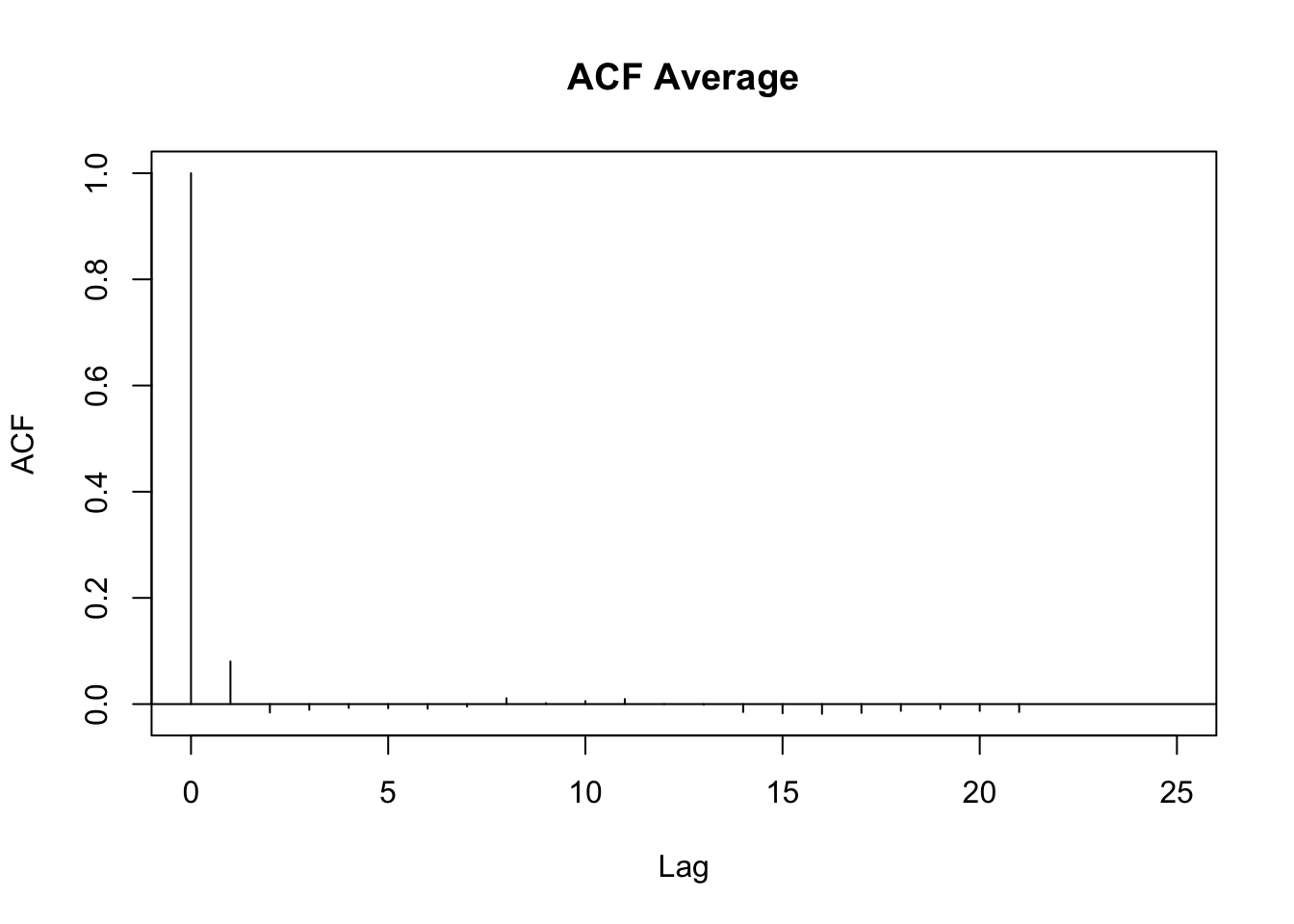
r1 <- start_value_rho(H2_model_1, 
                      plot=TRUE)

Code
H2_model_1 <- 
  bam(H2_form_1, 
      data = metric_participanthour, 
      discrete = TRUE,
      method = "fREML",
      nthreads = 10,
      rho = r1,
      AR.start = AR.start
      )

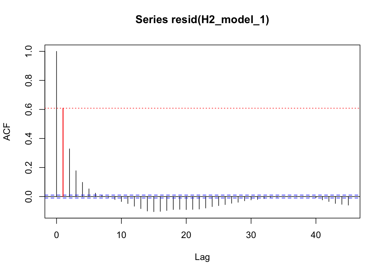
acf_resid(H2_model_1, split_pred = "AR.start")

Code
H2_summary_1 <- summary(H2_model_1)
H2_summary_1

Family: gaussian 
Link function: identity 

Formula:
lzMEDI ~ s(Time, k = 12) + s(Time, site, bs = "sz", k = 12) + 
    s(Time, Id, bs = "fs") + s(Id_date, bs = "re")

Parametric coefficients:
            Estimate Std. Error t value Pr(>|t|)    
(Intercept)  0.85202    0.02428   35.09   <2e-16 ***
---
Signif. codes:  0 '***' 0.001 '**' 0.01 '*' 0.05 '.' 0.1 ' ' 1

Approximate significance of smooth terms:
                edf  Ref.df       F p-value    
s(Time)       10.88   10.98 246.405  <2e-16 ***
s(Time,site)  67.22   74.28   5.909  <2e-16 ***
s(Time,Id)   743.18 1392.00   3.604  <2e-16 ***
s(Id_date)   350.78  801.00   0.846  <2e-16 ***
---
Signif. codes:  0 '***' 0.001 '**' 0.01 '*' 0.05 '.' 0.1 ' ' 1

R-sq.(adj) =  0.767   Deviance explained = 77.4%
fREML =  33250  Scale est. = 0.50672   n = 37603
Code
H2_model_1 |> glance()
# A tibble: 1 × 9
     df  logLik    AIC    BIC deviance df.residual  nobs adj.r.squared  npar
  <dbl>   <dbl>  <dbl>  <dbl>    <dbl>       <dbl> <int>         <dbl> <int>
1 1173. -31318. 64999. 75084.   20059.      36430. 37603         0.767  2327
Code
H2_model_1 |> appraise()

In [21]:
Code
Variance explained
Xp <- predict(H2_model_1, type = "terms")
variance <- apply(Xp, 2, var)
cor(Xp)
                  s(Time) s(Time,site)  s(Time,Id)   s(Id_date)
s(Time)      1.000000e+00 3.414971e-02 0.003808883 4.306839e-05
s(Time,site) 3.414971e-02 1.000000e+00 0.019654526 3.119813e-05
s(Time,Id)   3.808883e-03 1.965453e-02 1.000000000 1.432273e-01
s(Id_date)   4.306839e-05 3.119813e-05 0.143227274 1.000000e+00
Code
H2_R2 <- (variance/sum(variance)) |> enframe(value = "R2", name = "parameter")
H2_R2
# A tibble: 4 × 2
  parameter        R2
  <chr>         <dbl>
1 s(Time)      0.843 
2 s(Time,site) 0.0489
3 s(Time,Id)   0.0984
4 s(Id_date)   0.0100

Null model (H2_0)

In [22]:
Code
Null model
H2_model_0 <- 
  bam(H2_form_0, 
      data = metric_participanthour, 
      discrete = TRUE,
      method = "fREML",
      nthreads = 8
      )
Warning in gam.side(sm, X, tol = .Machine$double.eps^0.5): model has repeated
1-d smooths of same variable.
Code
r1 <- start_value_rho(H2_model_0, 
                      plot=TRUE)

Code
H2_model_0 <- 
  bam(H2_form_0, 
      data = metric_participanthour, 
      discrete = TRUE,
      method = "fREML",
      nthreads = 10,
      rho = r1,
      AR.start = AR.start
      )
Warning in gam.side(sm, X, tol = .Machine$double.eps^0.5): model has repeated
1-d smooths of same variable.
Code
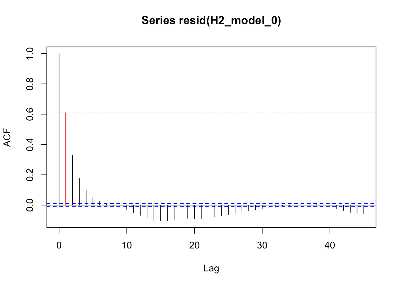
acf_resid(H2_model_0, split_pred = "AR.start")

Code
H2_summary_0 <- summary(H2_model_0)
H2_summary_0

Family: gaussian 
Link function: identity 

Formula:
lzMEDI ~ s(Time, k = 12) + s(Time, Id, bs = "fs") + s(Id_date, 
    bs = "re")

Parametric coefficients:
            Estimate Std. Error t value Pr(>|t|)    
(Intercept)  0.85639    0.03083   27.78   <2e-16 ***
---
Signif. codes:  0 '***' 0.001 '**' 0.01 '*' 0.05 '.' 0.1 ' ' 1

Approximate significance of smooth terms:
              edf  Ref.df       F p-value    
s(Time)     10.88   10.97 288.862  <2e-16 ***
s(Time,Id) 888.55 1408.00   5.477  <2e-16 ***
s(Id_date) 332.24  808.00   0.788  <2e-16 ***
---
Signif. codes:  0 '***' 0.001 '**' 0.01 '*' 0.05 '.' 0.1 ' ' 1

R-sq.(adj) =  0.768   Deviance explained = 77.5%
fREML =  33342  Scale est. = 0.5066    n = 37603
Code
H2_model_0 |> glance()
# A tibble: 1 × 9
     df  logLik    AIC    BIC deviance df.residual  nobs adj.r.squared  npar
  <dbl>   <dbl>  <dbl>  <dbl>    <dbl>       <dbl> <int>         <dbl> <int>
1 1233. -31283. 65039. 75594.   19961.      36370. 37603         0.768  2231
Code
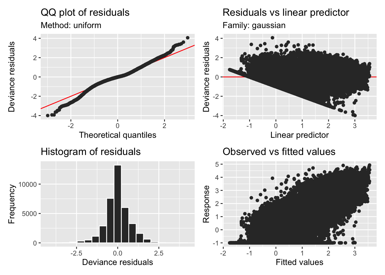
H2_model_0 |> appraise()

Code
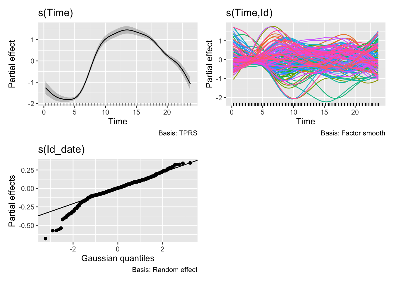
H2_model_0 |> draw()

Photoperiod model

In [23]:
Code
Photoperiod model
H2_model_phot <- 
  bam(H2_form_phot, 
      data = metric_participanthour, 
      discrete = TRUE,
      method = "fREML",
      nthreads = 10
      )

r1 <- start_value_rho(H2_model_phot, 
                      plot=TRUE)

Code
H2_model_phot <- 
  bam(H2_form_phot, 
      data = metric_participanthour, 
      discrete = TRUE,
      method = "fREML",
      nthreads = 10,
      rho = r1,
      AR.start = AR.start
      )

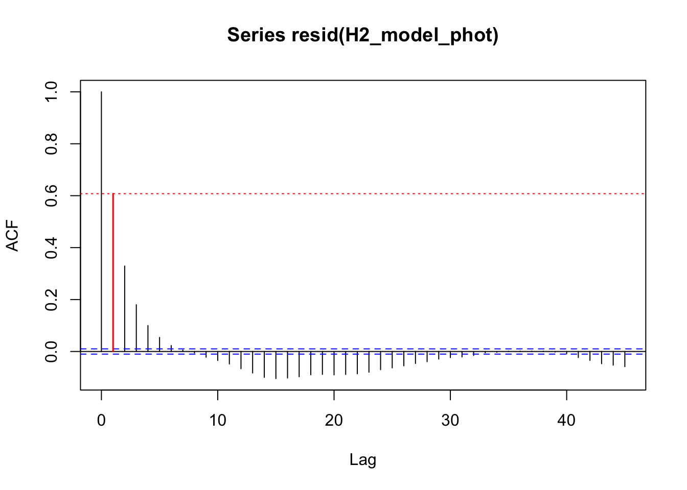
acf_resid(H2_model_phot, split_pred = "AR.start")

Code
H2_summary_phot <- summary(H2_model_phot)
H2_summary_phot

Family: gaussian 
Link function: identity 

Formula:
lzMEDI ~ s(Time, k = 12) + s(Time, site, bs = "sz", k = 12) + 
    s(Time, photoperiod.state, bs = "sz", k = 12) + s(Time, Id, 
    bs = "fs") + s(Id_date, bs = "re")

Parametric coefficients:
            Estimate Std. Error t value Pr(>|t|)    
(Intercept)  0.74254    0.03972    18.7   <2e-16 ***
---
Signif. codes:  0 '***' 0.001 '**' 0.01 '*' 0.05 '.' 0.1 ' ' 1

Approximate significance of smooth terms:
                              edf   Ref.df       F p-value    
s(Time)                    10.728   10.859 189.244  <2e-16 ***
s(Time,site)               65.227   72.442   5.496  <2e-16 ***
s(Time,photoperiod.state)   6.372    7.414   6.727  <2e-16 ***
s(Time,Id)                739.266 1392.000   3.565  <2e-16 ***
s(Id_date)                352.915  800.000   0.857  <2e-16 ***
---
Signif. codes:  0 '***' 0.001 '**' 0.01 '*' 0.05 '.' 0.1 ' ' 1

R-sq.(adj) =  0.767   Deviance explained = 77.5%
fREML =  33228  Scale est. = 0.50526   n = 37603
Code
H2_model_phot |> glance()
# A tibble: 1 × 9
     df  logLik    AIC    BIC deviance df.residual  nobs adj.r.squared  npar
  <dbl>   <dbl>  <dbl>  <dbl>    <dbl>       <dbl> <int>         <dbl> <int>
1 1176. -31290. 64951. 75068.   20014.      36427. 37603         0.767  2339
Code
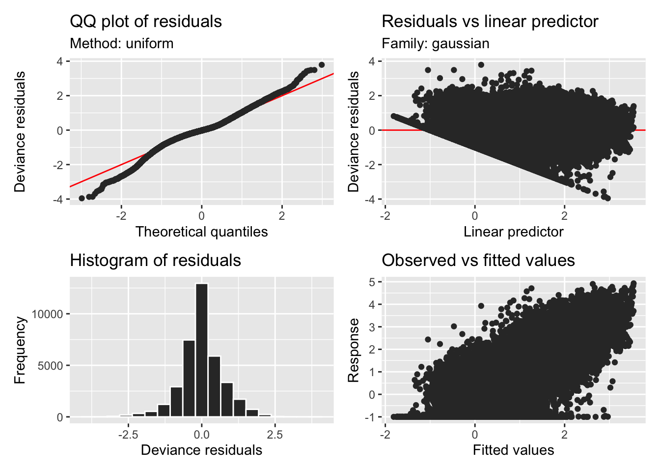
H2_model_phot |> appraise()

Code
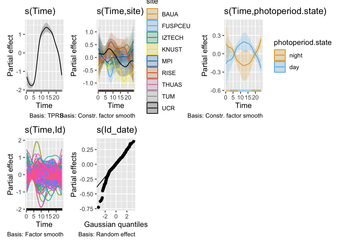
H2_model_phot |> draw()

Model comparison

In [24]:
Code
H2_AICs <- AIC(H2_model_1, H2_model_0, H2_model_phot)
H2_AICs |> as_tibble(rownames = "model") |> gt()
model df AIC
H2_model_1 1181.694 64998.72
H2_model_0 1236.679 65038.70
H2_model_phot 1185.327 64951.11

Since the ∆AIC of the base model against the null model is negative and lower than two (< -2), the base model is considered significantly better to explain the variance. The photoperiod model is even better and will be used henceforth.

In [25]:
Code
Variance explained
Xp <- predict(H2_model_phot, type = "terms")
variance <- apply(Xp, 2, var)

cor(Xp)
                                s(Time) s(Time,site) s(Time,photoperiod.state)
s(Time)                    1.0000000000 3.514529e-02               0.333261864
s(Time,site)               0.0351452880 1.000000e+00               0.070106573
s(Time,photoperiod.state)  0.3332618640 7.010657e-02               1.000000000
s(Time,Id)                 0.0043573936 2.104775e-02               0.020736766
s(Id_date)                -0.0001546661 1.489648e-05               0.001913475
                           s(Time,Id)    s(Id_date)
s(Time)                   0.004357394 -1.546661e-04
s(Time,site)              0.021047754  1.489648e-05
s(Time,photoperiod.state) 0.020736766  1.913475e-03
s(Time,Id)                1.000000000  1.441503e-01
s(Id_date)                0.144150283  1.000000e+00
Code
H2_R2 <- (variance/sum(variance)) |> enframe(value = "partial R2", name = "parameter")
H2_R2 |> gt() |> fmt_percent()
parameter partial R2
s(Time) 83.61%
s(Time,site) 4.87%
s(Time,photoperiod.state) 0.34%
s(Time,Id) 10.13%
s(Id_date) 1.05%

Model visualization

In [26]:
Code
prepare photoperiod model H2 plot
H2_site_data <- 
H2_model_phot |> 
  conditional_values(
    condition = list(Time = seq(0.25, 23.75, by = 0.5), "site", "photoperiod.state"),
    exclude = c("s(Time,Id)", "s(Id_date)")
    ) |> 
  mutate(across(c(.fitted, .lower_ci, .upper_ci),
                exp_zero_inflated)
  )

H2_site_data <-
metric_participanthour |> 
  Datetime2Time() |> 
  group_by(site, Time) |> 
  summarize(
    .groups = "drop_last",
    dawn = dawn |> as.numeric() |> mean(na.rm = TRUE)/3600,
    dusk = dusk |> as.numeric() |> mean(na.rm = TRUE)/3600
  ) |> 
  mutate(
    photoperiod.state = ifelse(between(Time, dawn, dusk), "day", "night")
  ) |> 
  select(-c(dawn, dusk)) |> 
  left_join(H2_site_data, by = c("site", "Time", "photoperiod.state"))

H2_site_data_phot <- 
H2_site_data |> 
  number_states(photoperiod.state) |> 
  filter(photoperiod.state == "night") |> 
  group_by(site, photoperiod.state.count) |> 
  summarize(xmin = min(Time),
            xmax = max(Time),
            .groups = "drop_last") |> 
    site_conv_mutate(rev = FALSE)
In [27]:
Code
Visualize photoperiod model H2
source("scripts/Brown_bracket.R")
Loading required package: legendry
Loading required package: ggtext
Code
H2_pred <- 
H2_site_data |> 
  site_conv_mutate(rev = FALSE) |>
  ggplot(aes()) +
  map(c(1,10,250, 10^4), 
          \(x) geom_hline(aes(yintercept = x), 
                          col = "grey", linetype = "dashed")
      ) +
  geom_rect(data = H2_site_data_phot ,
            aes(xmin = xmin, ymin = -Inf, ymax = Inf, xmax = xmax),
            alpha = 0.25, inherit.aes = FALSE) +
  geom_ribbon(aes(x = Time, ymin = .lower_ci, ymax = .upper_ci, fill = site), alpha = 0.5) +
  geom_line(aes(x = Time, y = .fitted, col = site), linewidth = 0.1) +
  geom_line(aes(x = Time, y = .fitted), linewidth = 1) +
  scale_fill_manual(values = melidos_colors) +
  scale_color_manual(values = melidos_colors) +
  theme_cowplot() +
  scale_y_continuous(trans = "symlog", breaks = c(0,1,10,100,250, 1000)) +
  scale_x_continuous(breaks = seq(0, 24, by = 6)) +
  coord_cartesian(xlim = c(0,24), ylim = c(0,10^4), expand = FALSE) +
  labs(y = "Melanopic EDI (lx)", x = "Local time (hrs)", fill = "Site", col = "Site") +
  facet_wrap(~site) +
  # guides( y = guide_axis_stack(Brown_bracket, "axis")) +
  gghighlight(
    label_key = site,
    label_params = list(x = 12, y = 4.5, force = 0, hjust = 0.25)
  ) +
  theme_sub_strip(background = element_blank(),
                  text = element_blank()) +
  theme(panel.spacing = unit(1, "lines"),
        plot.caption = element_textbox_simple())
  # labs(caption = Brown_caption)
In [28]:
Code
Visualize Individual
P_individual <- 
H2_model_phot |> 
  conditional_values(
    condition = list("Time", "Id"),
    exclude = c("s(Time,site)", "s(Id_date)", "s(Time,photoperiod.state)")
    ) |> 
  mutate(across(c(.fitted, .lower_ci, .upper_ci),
                exp_zero_inflated)
  ) |> 
  group_by(Id) |>
  select(-site) |> 
  separate_wider_delim(Id, delim = "_", names = c("site","Id")) |> 
  site_conv_mutate() |> 
  ggplot(aes(x = Time)) +
  map(c(1,10,250, 10^4), 
          \(x) geom_hline(aes(yintercept = x), col = "grey", linetype = "dashed")
      ) +
  # geom_ribbon(aes(ymin = .lower_ci, ymax = .upper_ci, group = Id), alpha = 0.025) +
  geom_line(aes(y = .fitted, group = interaction(Id, site), color = site), 
            linewidth = 1, alpha = 0.35) +
  theme_cowplot() +
  scale_color_manual(values = melidos_colors) +
  scale_y_continuous(trans = "symlog", breaks = c(0,1,10,100,250, 1000)) +
  scale_x_continuous(breaks = seq(0, 24, by = 6)) +
  coord_cartesian(xlim = c(0,24), ylim = c(0,1.5*10^4), expand = FALSE) +
  labs(y = "Melanopic EDI (lx)", x = "Local time (hrs)") +
  guides( y = guide_axis_stack(Brown_bracket, "axis"), color = "none") +
  theme(plot.caption = element_textbox_simple())
  # labs(caption = Brown_caption)
In [29]:
Code
prepare time model
H2_data <- 
H2_model_phot |> 
  conditional_values(
    condition = list(Time = seq(0.25, 23.75, by = 0.5), "photoperiod.state"),
    exclude = c("s(Time,site)", "s(Time,Id)", "s(Id_date)")
    ) |> 
  mutate(across(c(.fitted, .lower_ci, .upper_ci),
                exp_zero_inflated)
  )

H2_data <-
metric_participanthour |> 
  Datetime2Time() |> 
  group_by(Time) |> 
  summarize(
    .groups = "drop_last",
    dawn = dawn |> as.numeric() |> mean(na.rm = TRUE)/3600,
    dusk = dusk |> as.numeric() |> mean(na.rm = TRUE)/3600
  ) |> 
  mutate(
    photoperiod.state = ifelse(between(Time, dawn, dusk), "day", "night")
  ) |> 
  select(-c(dawn, dusk)) |> 
  left_join(H2_data, by = c("Time", "photoperiod.state"))

H2_data_phot <- 
H2_data |> 
  number_states(photoperiod.state) |> 
  filter(photoperiod.state == "night") |> 
  group_by(photoperiod.state.count) |> 
  summarize(xmin = min(Time),
            xmax = max(Time),
            .groups = "drop_last")
In [30]:
Code
Visualize Time
P_time <- 
H2_data |> 
  ggplot(aes(x = Time)) +
  map(c(1,10, 100, 250, 10^3), 
          \(x) geom_hline(aes(yintercept = x), col = "grey", linetype = "dashed")
      ) +
  geom_rect(data = H2_data_phot ,
            aes(xmin = xmin, ymin = -Inf, ymax = Inf, xmax = xmax),
            alpha = 0.25, inherit.aes = FALSE) +
  geom_ribbon(aes(ymin = .lower_ci, ymax = .upper_ci), alpha = 0.5) +
  geom_line(aes(y = .fitted), 
            linewidth = 1, alpha = 1) +
  theme_cowplot() +
  scale_y_continuous(trans = "symlog", breaks = c(0,1,10,100,250, 1000)) +
  scale_x_continuous(breaks = seq(0, 24, by = 6)) +
  coord_cartesian(xlim = c(0,24), ylim = c(0,1.5*10^3), expand = FALSE) +
  labs(y = "Melanopic EDI (lx)", x = "Local time (hrs)") +
  guides( y = guide_axis_stack(Brown_bracket, "axis"), color = "none") +
  theme(plot.caption = element_textbox_simple())
  # labs(caption = Brown_caption)
In [31]:
Code
Visualize model terms

P_terms <-
H2_model_phot |> 
  smooth_estimates(select = "s(Time,site)") |> 
  mutate(.lower_ci = .estimate -1.96*.se,
         .upper_ci = .estimate +1.96*.se,
         .fitted = .estimate,
         signif = .lower_ci > 0 | .upper_ci < 0,
         signif_id = consecutive_id(signif),
         .by = site) |> 
  site_conv_mutate(rev = FALSE) |>
  ggplot(aes()) +
  map(c(log10(c(0.1, 0.2, 0.5, 2, 5, 10))),
      \(x) geom_hline(yintercept = x, linewidth = 0.5, col = "grey", linetype = 2)) +
  geom_rect(data = H2_site_data_phot ,
            aes(xmin = xmin, ymin = -Inf, ymax = Inf, xmax = xmax),
            alpha = 0.25, inherit.aes = FALSE) +
  geom_ribbon(aes(x = Time, ymin = .lower_ci, ymax = .upper_ci, fill = site), alpha = 0.5) +
  geom_hline(yintercept = 0, linewidth = 1, linetype = 2) +
  geom_line(aes(x = Time, y = .fitted), 
            linewidth = 1) +
  geom_line(data = \(x) filter(x, signif),
            aes(x = Time, y = .fitted, group = signif_id), 
            col = "red", linewidth = 1) +
  scale_fill_manual(values = melidos_colors) +
  # scale_color_manual(values = c(melidos_colors)) +
  theme_cowplot() +
  scale_y_continuous(labels = expression(10^-1, 5^-1, 2^-1, "1  ", "2  ", "5  ", "10  "), 
                     breaks = log10(c(0.1, 0.2, 0.5, 1, 2, 5, 10)))+
  scale_x_continuous(breaks = seq(0, 24, by = 6)) +
  coord_cartesian(xlim = c(0,24), expand = FALSE) +
  guides(fill = "none") +
  labs(y = "Factor", x = "Local time (hrs)", fill = "Site") +
  facet_wrap(~site) +
  theme_sub_strip(background = element_blank(),
                  text = element_blank()) +
  theme(panel.spacing = unit(1, "lines"),
        plot.caption = element_textbox_simple())
In [32]:
Code
Combination of partial plots H2

((P_time / P_individual) | (H2_pred / P_terms)) +
  plot_annotation(tag_levels = "A", caption = Brown_caption,
                  theme = theme(plot.caption = element_textbox_simple())) +
  plot_layout()

Code

ggsave("figures/Fig4.pdf", height = 17, width = 13)

Interpretation

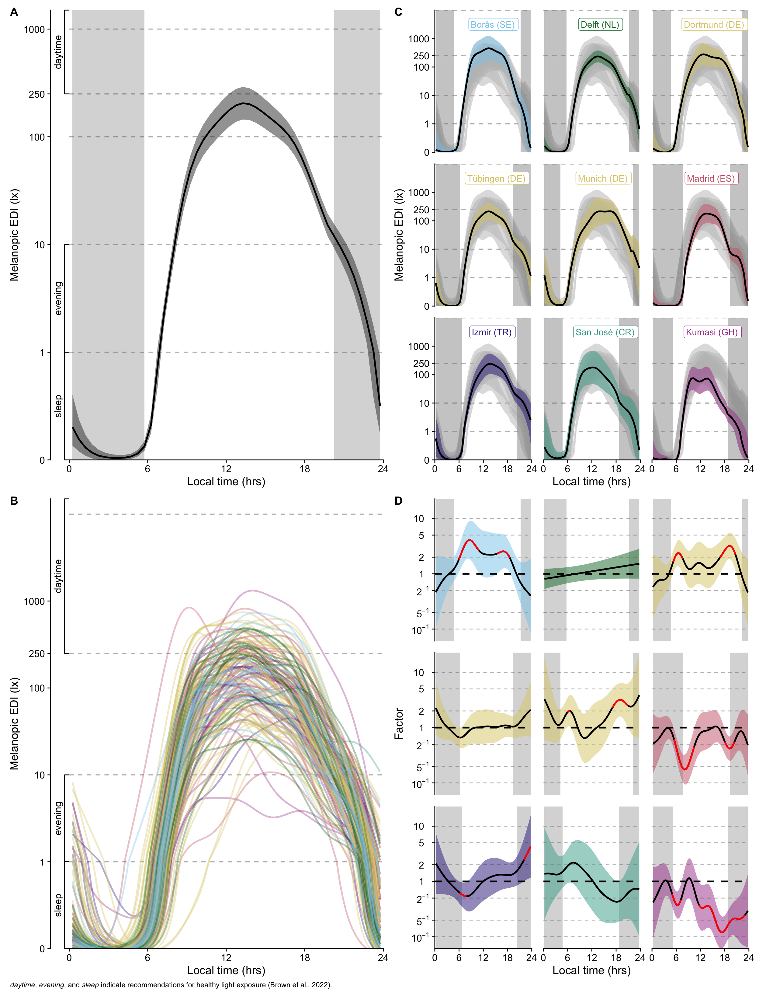
There is an overall trend of time and photoperiod (panel A). Daytime melanopic EDI light levels are < 100 lx in the morning and late afternoon, and between 100 and about 200 lx between late morning and early afternoon. During the evening, light levels are below 10 lx melanopic EDI, and generally below 1 lx at night.

Individual deviations from this trend vary greatly, especially during the day (panel B)

Model predictions (panel C) and deviations from the global trend (panel D) of each site shows specific differences:

  • Delft (NL), Tübingen (DE), and San José (CR) do not show significant deviations from the global trend. In the case of San José (CR) this is likely due to the small number of participants, as can be seen by the wide confidence interval compared to the other sites

  • Boras (SE), Dortmund (DE), and partially Munich (DE) show similar patterns of higher mel EDI in the hours after dawn and before dusk. The difference is about a factor 2-5 higher compared to the global trend.

  • Madrid (ES), Kumasi (GH), and Izmir (TR) have a significantly reduced mel EDI around dawn (factor 2-5 reduction)

  • Madrid (ES) and Kumasi (GH) have significantly reduced mel EDI around dusk (factor 2-5 reduction)

  • Izmir (TR) show significantly hightened melanopic EDI in the late evening (factor 2-5 increase)

  • Kumasi (GH) has significantly lower daytime illuminance both in the afternoon and after dusk (factor 2-5 reduction)

Session info

In [33]:
Code cell - Session info
sessionInfo()
R version 4.5.0 (2025-04-11)
Platform: aarch64-apple-darwin20
Running under: macOS 26.3.1

Matrix products: default
BLAS:   /Library/Frameworks/R.framework/Versions/4.5-arm64/Resources/lib/libRblas.0.dylib 
LAPACK: /Library/Frameworks/R.framework/Versions/4.5-arm64/Resources/lib/libRlapack.dylib;  LAPACK version 3.12.1

locale:
[1] en_US.UTF-8/en_US.UTF-8/en_US.UTF-8/C/en_US.UTF-8/en_US.UTF-8

time zone: Europe/Berlin
tzcode source: internal

attached base packages:
[1] stats     graphics  grDevices datasets  utils     methods   base     

other attached packages:
 [1] ggtext_0.1.2        legendry_0.2.4      gtsummary_2.5.0    
 [4] gghighlight_0.5.0   glmmTMB_1.1.14      gt_1.3.0           
 [7] broom.mixed_0.2.9.7 rlang_1.2.0         patchwork_1.3.2    
[10] gratia_0.11.2       itsadug_2.5         plotfunctions_1.5  
[13] broom_1.0.12        ggridges_0.5.7      cowplot_1.2.0      
[16] performance_0.16.0  lme4_2.0-1          Matrix_1.7-3       
[19] mgcv_1.9-4          nlme_3.1-168        LightLogR_0.10.0   
[22] melidosData_1.0.3   lubridate_1.9.5     forcats_1.0.1      
[25] stringr_1.6.0       dplyr_1.2.1         purrr_1.2.2        
[28] readr_2.2.0         tidyr_1.3.2         tibble_3.3.1       
[31] ggplot2_4.0.2       tidyverse_2.0.0    

loaded via a namespace (and not attached):
  [1] RColorBrewer_1.1-3   rstudioapi_0.18.0    jsonlite_2.0.0      
  [4] datawizard_1.3.0     magrittr_2.0.5       estimability_1.5.1  
  [7] farver_2.1.2         nloptr_2.2.1         rmarkdown_2.31      
 [10] fs_2.0.1             ragg_1.5.2           vctrs_0.7.3         
 [13] minqa_1.2.8          base64enc_0.1-6      effectsize_1.0.2    
 [16] htmltools_0.5.9      curl_7.0.0           haven_2.5.5         
 [19] sass_0.4.10          parallelly_1.47.0    htmlwidgets_1.6.4   
 [22] sandwich_3.1-1       emmeans_2.0.3        zoo_1.8-15          
 [25] TMB_1.9.21           commonmark_2.0.0     lifecycle_1.0.5     
 [28] pkgconfig_2.0.3      webshot2_0.1.2       R6_2.6.1            
 [31] fastmap_1.2.0        rbibutils_2.4.1      future_1.70.0       
 [34] digest_0.6.39        numDeriv_2016.8-1.1  furrr_0.4.0         
 [37] textshaping_1.0.5    labeling_0.4.3       timechange_0.4.0    
 [40] compiler_4.5.0       withr_3.0.2          S7_0.2.1-1          
 [43] backports_1.5.1      MASS_7.3-65          tools_4.5.0         
 [46] chromote_0.5.1       otel_0.2.0           glue_1.8.0          
 [49] promises_1.5.0       gridtext_0.1.6       grid_4.5.0          
 [52] see_0.13.0           generics_0.1.4       gtable_0.3.6        
 [55] labelled_2.16.0      tzdb_0.5.0           websocket_1.4.4     
 [58] hms_1.1.4            utf8_1.2.6           xml2_1.5.2          
 [61] ggrepel_0.9.8        pillar_1.11.1        markdown_2.0        
 [64] later_1.4.8          splines_4.5.0        lattice_0.22-7      
 [67] renv_1.1.4           tidyselect_1.2.1     juicyjuice_0.1.0    
 [70] knitr_1.51           reformulas_0.4.4     V8_8.1.0            
 [73] litedown_0.9         xfun_0.57            statmod_1.5.1       
 [76] stringi_1.8.7        yaml_2.3.12          boot_1.3-31         
 [79] ggokabeito_0.1.0     evaluate_1.0.5       codetools_0.2-20    
 [82] cli_3.6.6            tweedie_3.0.17       parameters_0.28.3   
 [85] systemfonts_1.3.2    Rdpack_2.6.6         processx_3.8.7      
 [88] mirai_2.6.1          Rcpp_1.1.1-1         globals_0.19.1      
 [91] coda_0.19-4.1        nanonext_1.8.2       parallel_4.5.0      
 [94] bayestestR_0.17.0    mvnfast_0.2.8        listenv_0.10.1      
 [97] broom.helpers_1.22.0 mvtnorm_1.3-7        scales_1.4.0        
[100] insight_1.5.0        cards_0.7.1