
#collect all the packages that are needed for the analysis
library(tidyverse)
library(cowplot)
library(gt)
library(gtsummary)
library(patchwork)
library(readxl)
library(ggsci)
library(ggcorrplot)
library(LightLogR)
library(rlang)
library(suntools)
library(legendry)
library(here)
library(lme4)
library(lmerTest)
library(broom.mixed)
library(lattice)
library(magrittr)
library(mgcv)
library(itsadug)
library(labelled)
library(ordinal)
library(ggtext)
library(magick)
library(ggh4x)
library(circular)
library(webshot2)
library(rnaturalearthdata)
library(gratia)

#source functions
source(here("functions/missing_data_table.R"))
source(here("functions/data_sufficient.R"))
source(here("functions/photoperiod.R"))
source(here("functions/table_lmer.R"))
source(here("functions/Inf_plots.R"))
source(here("functions/inference.R"))
source(here("functions/inference_table.R"))

#setting a seed for the date of generation to ensure reproducibility of random processes
seed <- 20241105

#if OpenMP is supported by the executing machine, analysis times for Research Question 2, Hypothesis 2, Patterns, can be sped up dramatically. If not supported, however, it distorts results dramatically and should not be used.
OpenMP_support <- TRUESupplement: analysis documentation
Physiologically-relevant light exposure and light behaviour in Switzerland and Malaysia
1 Preface
This is the analysis supplement to the publication “Physiologically-relevant light exposure and light behaviour in Switzerland and Malaysia”, as per the OSF Preregistration from 18 October 2024, version v1.0.1.
note: Creation of this analysis document based on its original script will fail, unless the recorded renv libraries are restored
In short, light exposure was measured in Basel, Switzerland, and Kuala Lumpur, Malaysia, for one month in 20 individuals per site. Additionally, questionnaires on sleep (PSQI) and light exposure behaviour (LEBA) were collected at specified times. The following hypotheses and research questions were formulated.
1.1 Research questions
RQ 1: Are there differences in objectively measured light exposure between the two sites, and if so, in which light metrics?
RQ 2: Are there differences in self-reported light exposure patterns using LEBA across time or between the two sites, and if so, in which questions/scores?
RQ 3 In general, how are light exposure and LEBA related and are there differences in this relationship between the two sites?
1.2 Hypotheses
For RQ 1, the following hypotheses will be addressed:
\(H1\): There are differences in light logger-derived light exposure intensity levels and duration of intensity between Malaysia and Switzerland.
\(H0_1\) : No differences between Malaysia and Switzerland.
\(H2\): There are differences in light logger-derived timing of light exposure between Malaysia and Switzerland.
\(H0_2\): No differences between Malaysia and Switzerland.
For RQ 2, the following hypotheses will be addressed:
\(H3\): There are differences in LEBA items and factors between Malaysia and Switzerland.
\(H0_3\): No differences between Malaysia and Switzerland.
\(H4\): LEBA scores vary over time within participants.
\(H0_4\): No differences between Malaysia and Switzerland.
For RQ 3, the following hypotheses will be addressed:
\(H5\): LEBA items correlate with preselected light-logger derived light exposure variables.
\(H0_5\): No correlation.
\(H6\): There is a difference between Malaysia and Switzerland on how well light-logger derived light exposure variables correlate with subjective LEBA items.
\(H0_6\): No differences between Malaysia and Switzerland.
2 Summary
This analysis shows several key differences and similarities between the two sites, Malaysia and Switzerland.
\(H1\): Swiss participants had significantly more time in daylight levels (above 1000 lx mel EDI) compared to Malaysian participants, and overall also stayed longer in healthy light levels during the day (above 250 lx mel EDI). While the photoperiod was longer in Switzerland than in Malaysia, this difference is still significant when adjusting for photoperiod, where the (unstandardized) effect size is almost a factor of two.
\(H2\): The brightest time of day was significantly brighter for Swiss participants compared to Malaysian participants, with a difference of about 0.5 log 10 units. The last time of day with light exposure was also significantly later in Switzerland compared to Malaysia, by about 1.5 hours, which can at least partly be attributed to the longer photoperiod. Swiss participants do, however, also avoid light exposure above 10 lx mel EDI significantly earlier than Malaysian participants, by about 1 hour and 10 minutes. Additionally, Swiss participants average about 1 log 10 unit mel EDI lower during evenings, compared to Malaysia. Finally, Swiss participants are about twice as often in a period of light above 250 lx mel EDI during the day.
\(H3\): LEBA questions and factors do not show a significant difference between Malaysia and Switzerland
\(H4\): Scores for most of the LEBA items are very stable over time. All 23 questions and 1 out of 5 factors do not vary significantly in more than 50% of participants.
\(H5\): LEBA items correlate with preselected light-logger derived light exposure variables in the Switzerland site, but not Malaysia. While exploratory analysis shows correlations in both sites, only Switzerland shows significant correlations after correction for multiple testing. Out of 84 correlations, 10 are significant in Switzerland. The effect size of those correlations is medium on average (r = 0.39).
\(H6\): There are few LEBA questions where the correlation coefficient differs significantly between sites. Specifically, these are the questions “I dim my mobile phone screen within 1 hour before attempting to fall asleep” & “I dim my computer screen within 1 hour before attempting to fall asleep”. While the correlation is positive with preselected light exposure metrics in Malaysia (r= 0.25, both), it is zero or negative in Switzerland (r = -0.01 and -0.15, respectively).
3 Setup
Data analysis is performed in R statistical software, mainly using the LightLogR R package, which is developed as part of the MeLiDos project. The document is rendered to HTML via Quarto.
The following packages are used for analysis
3.1 Global parameters
Here we set global parameters for the analysis. Except for the seed, these are specified in the preregistration document.
3.1.1 Coordinates and timezones of the sites
Coordinates are specified as latitude and longitude in decimal degrees. Timezones are chosen from the OlsonNames() function.
coordinates <- list(
#Basel Switzerland, University of Basel
malaysia = c(101.6009, 3.0650),
#Kuala Lumpur Malaysia, Monash University
switzerland = c(7.5839, 47.5585)
)

tzs <- list(
  malaysia = "Asia/Kuala_Lumpur",
  switzerland = "Europe/Zurich")
3.1.2 Illuminance threshold
The upper measurement threshold is set to 130,000 lx. While a lower threshold of 1 lx is specified in the preregistration, it will not be applied in the analysis, as variances of light levels below 1 lx are not relevant for the analysis parameters.
#set a maximum illuminance threshold in lx that is acceptable for the sensor values
illuminance_upper_th <- 1.3*10^5
3.1.3 Random metrics for the sensitivity analysis
The preregistration document specifies the procedure to define a threshold of missing data through a sensitivity analysis, based on three random metrics. These are defined here. The metrics are taken from Table 5 in the preregistration document with the exception of Interdaily Stability (IS), which cannot be calculated on a daily basis as the others.
#choosing three random metrics. This was the original script used to determine the metrics
# metrics <- c("TAT 250", "TAT 1000", "Period above 1000 lx", "M10m", "L5m", "IV", "LLiT 10", "LLit 250", "Frequency crossing threshold", "FLiT 1000", "LE", "M/P ratio")
#
# metrics_sample <-
#   sample(metrics, 3)
metrics_sample <- c("Llit 10","M/P ratio", "IV")
4 Import
4.1 Loading data in
4.1.1 Import light exposure data
The data sits in a folder structure that is organized by country and participant ID. Only .csv files that do not contain qualtrics in their file name from the subfolder Malaysia/ are imported. The data is imported using the Speccy import function of the LightLogR package, as this is the device used. The function automatically detects the participant ID from the file name. The timezone set is for Malaysia.
Note: Participant MY006 is missing from the data, as this participant lost the measurement device
#get all files in the Input/Malaysia folder that is inside a subfolder "MY001" to "MY020" and that does not contain "qualtrics" in the file name
base_folder <- "data/Malaysia"
ids <- sprintf("MY%03d", c(1:5, 7:20))
pattern <- "^(?!.*qualtrics).*\\.csv$"
all_folders <- file.path(base_folder, ids)
csv_files <-
  list.files(
    path = all_folders, pattern = "\\.csv$", full.names = TRUE, recursive = TRUE
    )
csv_files <- csv_files[!str_detect(csv_files, "qualtrics")]
id.pattern <- "MY[0-9]{3}"

#Import the data
data_malaysia <-
  import$Speccy(csv_files, tz = tzs[["malaysia"]], auto.id = id.pattern)
Successfully read in 733'908 observations across 19 Ids from 40 Speccy-file(s).
Timezone set is Asia/Kuala_Lumpur.
The system timezone is Europe/Berlin. Please correct if necessary!

First Observation: 2023-11-20 10:13:58
Last Observation: 2023-12-30 00:30:00
Timespan: 40 days

Observation intervals:
   Id    interval.time              n pct
 1 MY001 60s (~1 minutes)       43330 100%
 2 MY001 65s (~1.08 minutes)        1 0%
 3 MY002 59s                        1 0%
 4 MY002 60s (~1 minutes)       22189 100%
 5 MY002 61s (~1.02 minutes)        1 0%
 6 MY002 9978s (~2.77 hours)        1 0%
 7 MY002 17965s (~4.99 hours)       1 0%
 8 MY002 32323s (~8.98 hours)       1 0%
 9 MY002 1202366s (~1.99 weeks)     1 0%
10 MY003 60s (~1 minutes)       43195 100%
# ℹ 35 more rows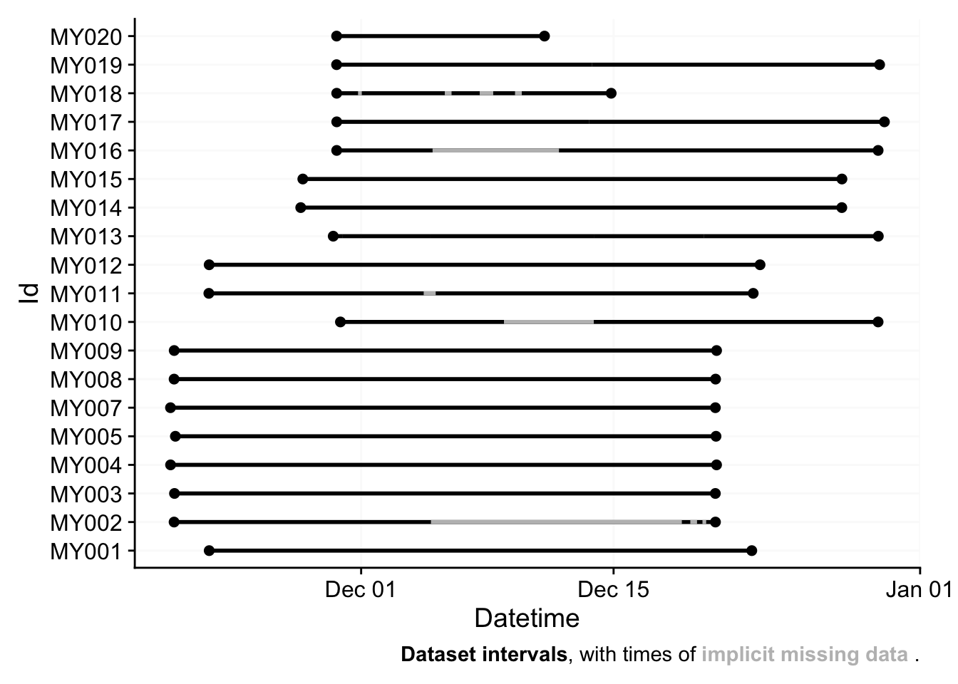
#renaming the wavelength columns
data_malaysia <-
  data_malaysia %>%
  rename_with(\(x) {
    paste0("WL_", x) %>% str_replace("[.][.][.]", "")
  },
  `...380`:`...780`
  )
4.1.2 Missing data
The summary shows that all data were collected approximately at the same time, and about half of them are without gaps. The next section will make implicit gaps explicit. This will be done by creating a regular time series from first until last day of measurement. Minutes without an observation will be filled with NA.
#check for gaps (implicit missing data)
data_malaysia %>% gap_finder()
#confirm that the regular epoch is 1 minute
data_malaysia %>% dominant_epoch()
# A tibble: 19 × 3
Id dominant.epoch group.indices
<fct> <Duration> <int>
1 MY001 60s (~1 minutes) 1
2 MY002 60s (~1 minutes) 2
3 MY003 60s (~1 minutes) 3
4 MY004 60s (~1 minutes) 4
5 MY005 60s (~1 minutes) 5
6 MY007 60s (~1 minutes) 6
7 MY008 60s (~1 minutes) 7
8 MY009 60s (~1 minutes) 8
9 MY010 60s (~1 minutes) 9
10 MY011 60s (~1 minutes) 10
11 MY012 60s (~1 minutes) 11
12 MY013 60s (~1 minutes) 12
13 MY014 60s (~1 minutes) 13
14 MY015 60s (~1 minutes) 14
15 MY016 60s (~1 minutes) 15
16 MY017 60s (~1 minutes) 16
17 MY018 60s (~1 minutes) 17
18 MY019 60s (~1 minutes) 18
19 MY020 60s (~1 minutes) 19#bring data into a regular time series of 1 minute
data_malaysia_temp <-
data_malaysia %>% mutate(Datetime = round_date(Datetime, "1 minute"))
#check that no Datetime is present twice after rounding
stopifnot("At least one datetime is present twice after rounding" =
data_malaysia_temp$Datetime %>% length() %>% {. == nrow(data_malaysia)}
)
#show a summary of implicitly missing data
implicitly_missing_summary(data_malaysia_temp,
"Implicitly missing data in the Malaysia dataset", 60)| min | max | median | mean | total | |
|---|---|---|---|---|---|
| Number of gaps | 0 | 7 | 0 | 1 | 21 |
| Duration missed by available data points | 0 days | 14 days | 0 days | 1 day | 29 days |
| Duration covered by available data points | 11 days | 30 days | 30 days | 26 days | 509 days |
| Number of missing data points | 0 | 21,040 | 0 | 2,200 | 41,796 |
| Number of available data points | 16,604 | 43,996 | 43,212 | 38,627 | 733,908 |
| Percentage of missing data points | 0.0% | 48.7% | 0.0% | 5.4% | 5.4% |
| min, max, median, mean, and total values for 19 participants | |||||
#make implicit gaps explicit
data_malaysia <- data_malaysia_temp %>% gap_handler(full.days = TRUE)
#check for gaps
data_malaysia %>% gap_finder()
#remove the temporary dataframe
rm(data_malaysia_temp)

#show values above the photopic illuminance thresholds
data_malaysia %>%
  filter(Photopic.lux > illuminance_upper_th) %>%
  select(Id, Datetime, Photopic.lux, MEDI) %>%
  gt(caption =
paste("Values above", illuminance_upper_th, "lx photopic illuminance"))| Datetime | Photopic.lux | MEDI |
|---|---|---|
| MY014 | ||
| 2023-12-22 14:26:00 | 133096.7 | 132775.7 |
#apply the filter for the upper illuminance threshold
data_malaysia <-
data_malaysia %>%
  filter(Photopic.lux <= illuminance_upper_th | is.na(Photopic.lux)) %>%
  gap_handler()

#set illuminance values to 0.1 if they are below 1 lux (as the sensor does not measure below 1 lux, but 0.1 lx can be logarithmically transformed)
data_malaysia <-
  data_malaysia %>%
  mutate(MEDI = ifelse(Photopic.lux < 1, 0.1, MEDI))

#show a summary of data missing in general
data_malaysia %>% filter(!is.na(MEDI)) %>%
  implicitly_missing_summary(
                           "Missing data in the Malaysia dataset overall",
60)| min | max | median | mean | total | |
|---|---|---|---|---|---|
| Number of gaps | 0 | 7 | 0 | 1 | 22 |
| Duration missed by available data points | 0 days | 14 days | 0 days | 1 day | 29 days |
| Duration covered by available data points | 11 days | 30 days | 30 days | 26 days | 509 days |
| Number of missing data points | 0 | 21,040 | 0 | 2,200 | 41,797 |
| Number of available data points | 16,604 | 43,996 | 43,211 | 38,627 | 733,907 |
| Percentage of missing data points | 0.0% | 48.7% | 0.0% | 5.4% | 5.4% |
| min, max, median, mean, and total values for 19 participants | |||||
4.1.3 Import LEBA data
In this section the LEBA data is imported. The data is stored in a MYXXX_qualtrics.csv file within each participant’s folder. It contains questionnaire data. Days are coded 1 to X (X being the last day), so the dates need to be connected with the dates from the light data.
#Import the data
leba_folders <- file.path(base_folder, ids)
pattern <- "qualtrics\\.csv$"
leba_files <-
  list.files(path = leba_folders, pattern = pattern, full.names = TRUE)

leba_malaysia <-
  read_csv(leba_files, id = "file.path") %>%
  mutate(Id = str_extract(file.path, id.pattern) %>% as.factor(),
         Day = parse_number(`...1`)
         ) %>%
  select(Id, Day, starts_with("leba"))

#extract the questions from the data
leba_questions <- leba_malaysia[1,-c(1,2)] %>% unlist()

#set the factor levels for leba
leba_levels <- c("Never", "Rarely", "Sometimes", "Often", "Always")

#drop the first row and set the factor levels
leba_malaysia <-
  leba_malaysia %>%
  drop_na(Day) %>%
  mutate(across(starts_with("leba"), ~ factor(.x, levels = leba_levels)))

#drop rows with NA
leba_malaysia <- leba_malaysia %>% drop_na()

#set variable labels
var_label(leba_malaysia) <- leba_questions %>% as.list()
4.1.4 Import light exposure data
The Swiss data are structured by participant folders, with one or more .csv files by participant.
#get all files in the data/Basel/Speccy folder that is inside a subfolder "ID01" to "ID20" and in those a .csv file
base_folder <- "data/Basel/Speccy"
subfolders <- sprintf("ID%02d", 1:20)
pattern <- "\\.csv$"
all_folders <- file.path(base_folder, subfolders)
csv_files <- list.files(path = all_folders, pattern = pattern, full.names = TRUE, recursive = TRUE)
id.pattern <- "ID\\d{2}"

#Import the data
data_switzerland <- import$Speccy(csv_files, tz = tzs[["switzerland"]], auto.id = id.pattern)
Successfully read in 799'088 observations across 20 Ids from 49 Speccy-file(s).
Timezone set is Europe/Zurich.
The system timezone is Europe/Berlin. Please correct if necessary!

First Observation: 2023-07-17 17:30:00
Last Observation: 2023-10-18 14:10:36
Timespan: 93 days

Observation intervals:
   Id    interval.time              n pct
 1 ID01  60s (~1 minutes)       35968 100%
 2 ID01  36180s (~10.05 hours)      1 0%
 3 ID01  67260s (~18.68 hours)      1 0%
 4 ID01  302520s (~3.5 days)        1 0%
 5 ID02  60s (~1 minutes)       43530 100%
 6 ID02  1538s (~25.63 minutes)     1 0%
 7 ID03  60s (~1 minutes)       43873 100%
 8 ID03  1488s (~24.8 minutes)      1 0%
 9 ID03  43282s (~12.02 hours)      1 0%
10 ID04  60s (~1 minutes)       41554 100%
# ℹ 39 more rows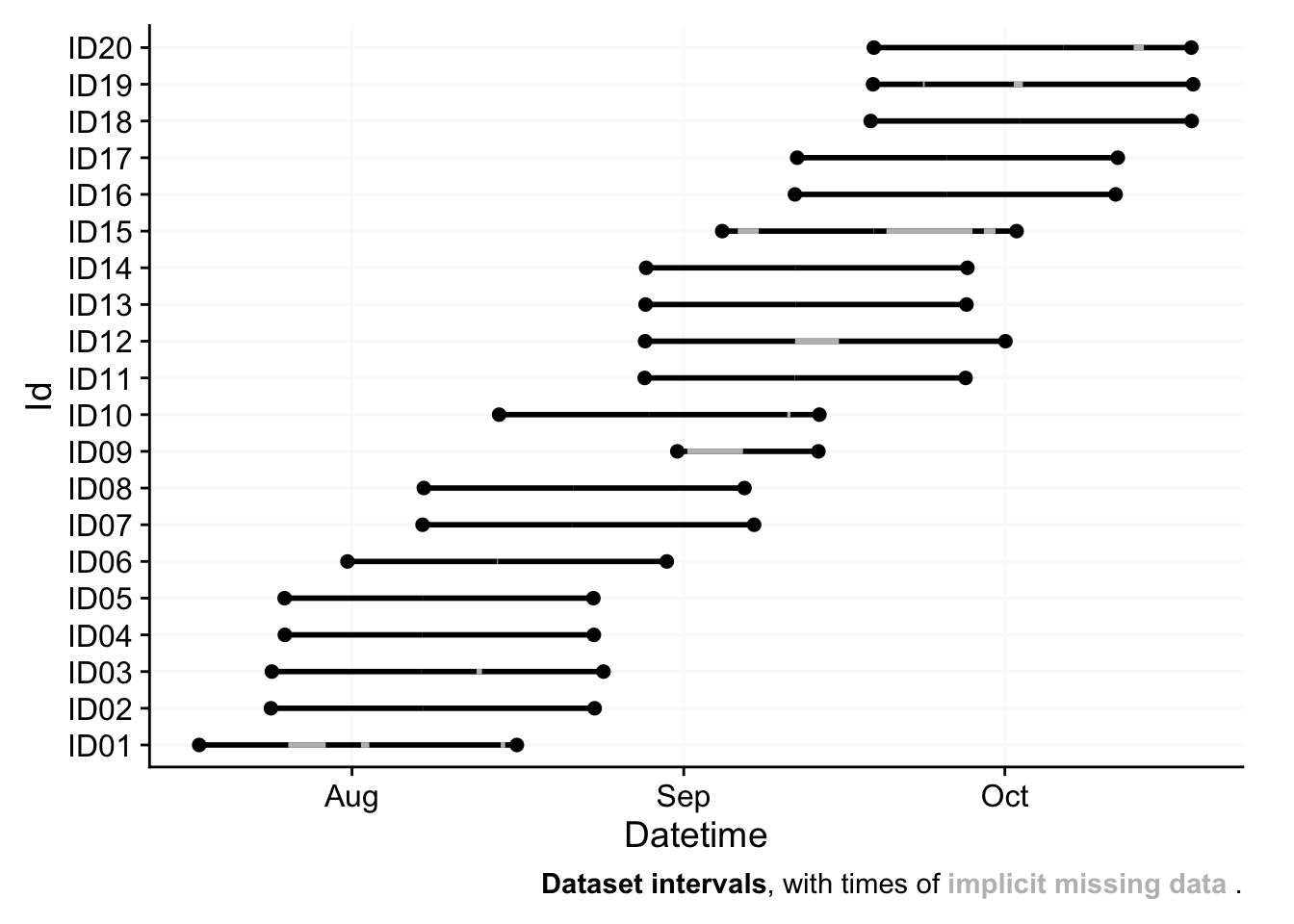
#renaming the wavelength columns
data_switzerland <-
  data_switzerland %>%
  rename_with(\(x) {
    paste0("WL_", x) %>% str_replace("[.][.][.]", "")
  },
  `...380`:`...780`
  )
4.1.5 Missing data
The overview suggests there is implicit missing data, which will be cleaned the following way:
#check for gaps (implicit missing data)
data_switzerland %>% gap_finder()
#confirm that the regular epoch is 1 minute
data_switzerland %>% dominant_epoch()
# A tibble: 20 × 3
Id dominant.epoch group.indices
<fct> <Duration> <int>
1 ID01 60s (~1 minutes) 1
2 ID02 60s (~1 minutes) 2
3 ID03 60s (~1 minutes) 3
4 ID04 60s (~1 minutes) 4
5 ID05 60s (~1 minutes) 5
6 ID06 60s (~1 minutes) 6
7 ID07 60s (~1 minutes) 7
8 ID08 60s (~1 minutes) 8
9 ID09 60s (~1 minutes) 9
10 ID10 60s (~1 minutes) 10
11 ID11 60s (~1 minutes) 11
12 ID12 60s (~1 minutes) 12
13 ID13 60s (~1 minutes) 13
14 ID14 60s (~1 minutes) 14
15 ID15 60s (~1 minutes) 15
16 ID16 60s (~1 minutes) 16
17 ID17 60s (~1 minutes) 17
18 ID18 60s (~1 minutes) 18
19 ID19 60s (~1 minutes) 19
20 ID20 60s (~1 minutes) 20#bring data into a regular time series of 1 minute
data_switzerland_temp <-
data_switzerland %>% mutate(Datetime = round_date(Datetime, "1 minute"))
#check that no Datetime is present twice after rounding
stopifnot("At least one datetime is present twice after rounding" =
data_switzerland_temp$Datetime %>% length() %>% {. == nrow(data_switzerland)}
)
#show a summary of implicitly missing data
implicitly_missing_summary(data_switzerland_temp,
"Implicitly missing data in the Swiss dataset", 60)| min | max | median | mean | total | |
|---|---|---|---|---|---|
| Number of gaps | 1 | 4 | 1 | 1 | 29 |
| Duration missed by available data points | <1 day | 11 days | <1 day | 1 day | 28 days |
| Duration covered by available data points | 7 days | 30 days | 29 days | 27 days | 554 days |
| Number of missing data points | 20 | 16,017 | 40 | 2,034 | 40,680 |
| Number of available data points | 11,476 | 44,588 | 42,974 | 39,954 | 799,088 |
| Percentage of missing data points | 0.0% | 40.4% | 0.1% | 5.9% | 4.8% |
| min, max, median, mean, and total values for 20 participants | |||||
#make implicit gaps explicit
data_switzerland <- data_switzerland_temp %>% gap_handler(full.days = TRUE)
#check for gaps
data_switzerland %>% gap_finder()
#remove the temporary dataframe
rm(data_switzerland_temp)

#show values above the photopic illuminance thresholds
data_switzerland %>%
  filter(Photopic.lux > illuminance_upper_th) %>%
  select(Id, Datetime, Photopic.lux, MEDI) %>%
  gt(caption =
paste("Values above", illuminance_upper_th, "lx photopic illuminance"))| Datetime | Photopic.lux | MEDI |
|---|---|---|
| ID01 | ||
| 2023-08-07 15:10:00 | 1.302806e+05 | 1.345450e+05 |
| ID03 | ||
| 2023-08-09 16:49:00 | 1.350211e+05 | 1.347234e+05 |
| ID07 | ||
| 2023-09-05 13:56:00 | 1.455028e+05 | 1.298996e+05 |
| 2023-09-06 13:35:00 | 1.370206e+05 | 1.223984e+05 |
| ID18 | ||
| 2023-09-26 19:28:00 | 1.267747e+27 | 9.370563e+23 |
| 2023-09-26 19:32:00 | 1.267747e+27 | 9.370563e+23 |
| 2023-09-26 19:34:00 | 1.575518e+15 | 1.613236e+12 |
| 2023-09-26 19:36:00 | 1.267747e+27 | 9.370563e+23 |
#apply the filter for the upper illuminance threshold
data_switzerland <-
data_switzerland %>%
  filter(Photopic.lux <= illuminance_upper_th | is.na(Photopic.lux)) %>%
  gap_handler()

#set illuminance values to 0.1 if they are below 1 lux (as the sensor does not measure below 1 lux, but 0.1 lx can be logarithmically transformed)
data_switzerland <-
  data_switzerland %>%
  mutate(MEDI = ifelse(Photopic.lux < 1, 0.1, MEDI))

#show a summary of data missing in general
data_switzerland %>% filter(!is.na(MEDI)) %>%
  implicitly_missing_summary(
                           "Missing data in the Swiss dataset overall",
60)| min | max | median | mean | total | |
|---|---|---|---|---|---|
| Number of gaps | 1 | 4 | 1 | 2 | 35 |
| Duration missed by available data points | <1 day | 11 days | <1 day | 1 day | 28 days |
| Duration covered by available data points | 7 days | 30 days | 29 days | 27 days | 554 days |
| Number of missing data points | 21 | 16,017 | 44 | 2,035 | 40,698 |
| Number of available data points | 11,476 | 44,586 | 42,974 | 39,954 | 799,070 |
| Percentage of missing data points | 0.0% | 40.4% | 0.1% | 5.9% | 4.8% |
| min, max, median, mean, and total values for 20 participants | |||||
4.1.6 Import LEBA data
In this section the LEBA data is imported. The data is stored in the REDCap_CajochenASEAN_DATA_2023-10-30_1215.csv file in the REDCap folder. It contains questionnaire data. Days are coded 1 to X (X being the last day), so the dates need to be connected with the dates from the light data.
The basel data also contains more columns coded with leba than the Malaysia data. Only the ones contained in both locations will be chosen.
#Import the data
leba_folders <- "data/Basel/REDCap"
leba_file <- "REDCap_CajochenASEAN_DATA_2023-10-30_1215.csv"
leba_files <- paste(leba_folders, leba_file, sep = "/")

leba_switzerland <-
  read_csv(leba_files, id = "file.path") %>%
  mutate(Day = parse_number(redcap_event_name)) %>%
  fill(code) %>%
  select(Id = code, Day, starts_with("leba"))

#replace the small factor f to an uppercase F
names(leba_switzerland) <-
names(leba_switzerland) %>% str_replace_all("f(\\d)", "F\\1")

#set the factor levels for leba
leba_levels <- c("Never", "Rarely", "Sometimes", "Often", "Always")

#get the column names
colnames_leba <- names(leba_questions)

#merge the columns with the same name, where one ends with _2, unite the dates
leba_switzerland <-
  colnames_leba %>%
  reduce(
    \(y,x)
    y %>%
      unite(
        col = !!x,
        matches(x), matches(paste0(x, "_2")),
        na.rm = TRUE
        ),
    .init = leba_switzerland
    ) %>%
  unite(col = Datetime,
        leba_weekly_timestamp, leba_end_timestamp,
        na.rm = TRUE) %>%
  select(Id, Day, Datetime, starts_with("leba_f")) %>%
  mutate(across(starts_with("leba"),
           ~ factor(.x, levels = 1:5, labels = leba_levels))) %>%
  drop_na()

#set variable labels
var_label(leba_switzerland) <- leba_questions %>% as.list()
As the codes in REDCap and the Ids in the light data do not match, we need to enlist a conversion table.
file_conv <- "data/Basel/Participant List Anonymised.xlsx"
#import the conversion file
conv_switzerland <-
  read_xlsx(file_conv) %>%
  select(ID, Code) %>%
  mutate(ID = sprintf("ID%02d", ID))

#one Id in the conversion file does not match with a code in the Leba data
# conversion file: 1998NABR
# leba data: 1999NABR
# we correct the conversion file according to the leba data
conv_switzerland <-
  conv_switzerland %>%
  mutate(Code = if_else(Code == "1998NABR", "1999NABR", Code))

#add the conversion table to the leba data
leba_switzerland <-
  leba_switzerland %>%
  left_join(conv_switzerland, by = c("Id" = "Code")) %>%
  select(-Id) %>%
  rename(Id = ID) %>%
  drop_na(starts_with("leba")) %>%
  dplyr::relocate(Id, .before = 1)
4.1.7 Determining the cutoff for required data of participant-days
Each participant-day is required to have at least a set number of datapoints or it will be excluded from the analysis. The procedure on how to determine this cutoff is described in the preregistration document. Data will be aggregated to hourly values and threshold values in 1 hour instances tested, i.e. 1/24 of a day. The minimum threshold is set to 3/24, as calculating the IV requires 3 data points. Participants MY004, MY009, and MY012 were chosen randomly to determine the threshold.
This section took about 40 hrs compute time on a M2 Macbook Pro, 64 GB RAM. Thus for normal execution, bootstrapped results are stored in data/processed, and only analysed here.
#choosing three participants without missing data.

# n_participants <- 3
#
# coverage <-
# data_malaysia %>% filter(!is.na(MEDI)) %>%
#     summarize(
#       length_no_complete = length(Datetime),
#       length_days = length_no_complete/60/24
#     )
#
# random_participants <-
# suppressWarnings({
#   data_malaysia %>%
#     filter(!is.na(MEDI)) %>%
#     gap_finder(gap.data = TRUE, silent = TRUE) %>%
#         group_by(Id, .drop = FALSE) %>%
#         summarise(gaps = max(gap.id)
#         ) %>%
#         mutate(gaps = ifelse(gaps == -Inf, 0, gaps))
#     }) %>%
#   left_join(coverage, by = "Id") %>%
#   filter(gaps == 0 & length_days >=29) %>%
#   slice_sample(n = n_participants) %>%
#   pull(Id)

random_participants <- c("MY004", "MY009", "MY012")
The chosen metrics are Llit 10, M/P ratio, IV, the chosen participants are MY004, MY009, MY012.
4.1.7.1 Calculating metrics
#filter the dataset
subset_malaysia <-
  data_malaysia %>%
  filter(Id %in% random_participants)

#remove the (incomplete) first and last day of measurement
subset_malaysia <-
  subset_malaysia %>%
  aggregate_Datetime(unit = "1 hour") %>%
  mutate(Day = date(Datetime)) %>%
  filter_Datetime(filter.expr =
                    Day > min(Day) & Day < (max(Day)-days(1)))

subset_malaysia %>% gg_overview()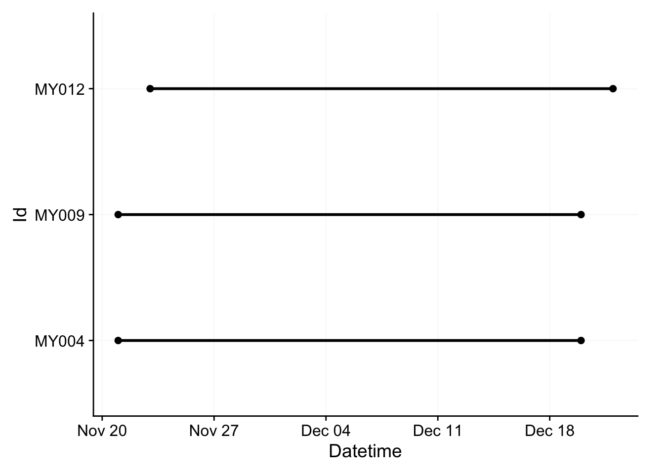
#metrics function
metrics_function <- function(dataset) {
  dataset %>%
    summarize(
    MP_ratio = mean(MEDI)/mean(Photopic.lux),
            LLiT10 =
              timing_above_threshold(
              MEDI, Datetime, "below", 10, as.df = TRUE),
            IV = intradaily_variability(MEDI, Datetime),
            .groups = "drop_last"
            ) %>%
  unnest_wider(col = c(LLiT10)) %>%
  select(-first_timing_below_10, -mean_timing_below_10) %>%
    mutate(last_timing_below_10 =
             hms::as_hms(last_timing_below_10) %>% as.numeric)
  }

# calculate the metrics
subset_metrics <-
  subset_malaysia %>%
  group_by(Day, .add = TRUE) %>%
  metrics_function() %>%
      pivot_longer(
        cols = -c(Day, Id), names_to = "metric", values_to = "value") %>%
  group_by(metric, Id) %>%
  summarize(
    mean = mean(value, na.rm = TRUE),
    sd = stats::sd(value, na.rm = TRUE),
    se = sd/sqrt(n()-1),
    qlower = quantile(value, 0.4, na.rm = TRUE),
    qupper = quantile(value, 0.6, na.rm = TRUE),
    upper_Acc = max(value, na.rm = TRUE),
    lower_Acc = min(value, na.rm = TRUE),
    .groups = "drop"
  )
4.1.7.2 creating bootstraps
#for each participant-day, remove the specified number of datapoints
#and calculate the metrics
bootstrap_basis <-
  subset_malaysia %>%
  group_by(Id, Day) %>%
  select(Id, Day, Datetime, MEDI, Photopic.lux)
#thresholds for the bootstrapping
n_bootstraps <- 2
thresholds <- seq(1, 21, by = 1)
#create the bootstraps
#this is commented out in production, because the process takes about 40+ hours of compute-time
#creating 5000 files with 2 bootstraps each
# (1:(0.5*10^4)) %>% walk(\(x) {
#
# bootstraps <-
# tibble(
# threshold = rep(thresholds, each = n_bootstraps),
# bootstrap_id = seq_along(threshold),
# data =
# threshold %>% map(\(x) bootstrap_basis %>% slice_sample(n = 24-x))
# ) %>%
# unnest(data) %>%
# group_by(threshold, bootstrap_id, Id, Day) %>%
# arrange(Datetime, .by_group = TRUE) %>%
# metrics_function() %>%
# pivot_longer(cols = -c(threshold, bootstrap_id, Id, Day), names_to = "metric", values_to = "value")
# #
# #save these to disk
# save(bootstraps, file = sprintf("data/processed/bootstrap%04d.RData", x))
#
# })#then bring the bootstraps together to one file
# bootdata <- tibble()
# walk(1:5000, \(x) {
# load(sprintf("data/processed/bootstrap%04d.RData", x))
# bootdata <<- bind_rows(bootdata, bootstraps)
# })
# bootstraps <- bootdata
# save(bootstraps, file = "data/processed/bootstraps.RData")#bootstrap condensation
# source("scripts/bootstrap_condensation.R")#if previous chunks for bootstrapping are executed, comment this chunk out
load(file = "data/processed/bootstraps.RData")#the bootstraps are now summarized at the metric per participant level for each threshold. These are compared to the original metrics and their bounds. bootstrap condensation in the script "scripts/bootstrap_condensation.R"
bootstrap_comparison <-
bootstraps %>%
left_join(subset_metrics, by = c("Id", "metric"))
#visualize the results
bootstrap_comparison %>%
ggplot(aes(x = threshold)) +
geom_ribbon(aes(ymin = (mean - 2*se), ymax = (mean + 2*se)),
fill = "steelblue", alpha = 0.4) +
geom_hline(data = subset_metrics, aes(yintercept=mean), color = "steelblue") +
geom_errorbar(
aes(ymin = lower_bs1, ymax = upper_bs1), linewidth = 0.5, width = 0) +
geom_errorbar(aes(ymin = lower_bs2, ymax = upper_bs2),
linewidth = 0.25, width = 0) +
geom_point(aes(y=mean_bs,
col = ((mean - 2*se) <= lower_bs3 & upper_bs3 <= (mean + 2*se)))) +
facet_wrap(Id~metric, scales = "free") +
theme_minimal() +
labs(x = "Hours missing from the day (Threshold)", y = "Metric value", col = "Within Range") +
theme(legend.position = "bottom")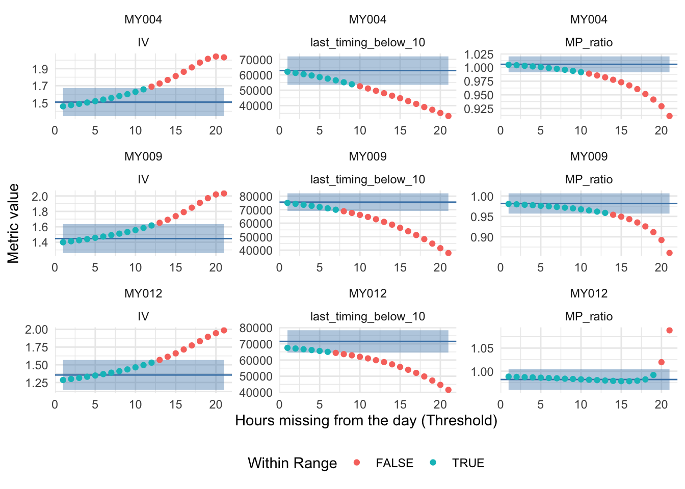
The most conservative threshold is chosen based on participant MY009 and the metric last_timing_below_10, which allows up to 6 hours of missing data per day, i.e. 25.00%. For this assumption to hold, the data must be missing at random hours of the day.
missing_threshold <- 18/244.1.8 Remove participant-days with insufficient data
The threshold determined in Section 4.1.7 is used to remove participant-days with insufficient data.
#mark data that is above the upper illuminance threshold
data_malaysia <-
  data_malaysia %>%
  group_by(Day = date(Datetime), .add = TRUE) %>%
    mutate(marked_for_removal =
             !data_sufficient(MEDI, missing_threshold),
           .before = 1
          ) %>%
  ungroup(Day)

#display the final malaysia dataset prior to analysis, where each dot marks the start/end of a day
data_malaysia %>%
  filter(!marked_for_removal) %>%
  group_by(Day, .add = TRUE) %>%
  gg_overview()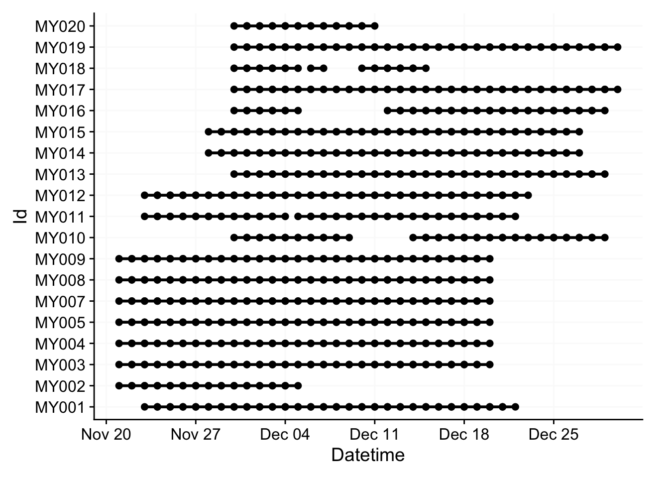
#mark data that is above the upper illuminance threshold
data_switzerland <-
  data_switzerland %>%
  group_by(Day = date(Datetime), .add = TRUE) %>%
    mutate(marked_for_removal =
             !data_sufficient(MEDI, missing_threshold),
           .before = 1
          ) %>%
  ungroup(Day)

#display the final malaysia dataset prior to analysis, where each dot marks the start/end of a day
data_switzerland %>%
  filter(!marked_for_removal) %>%
  group_by(Day, .add = TRUE) %>%
  gg_overview()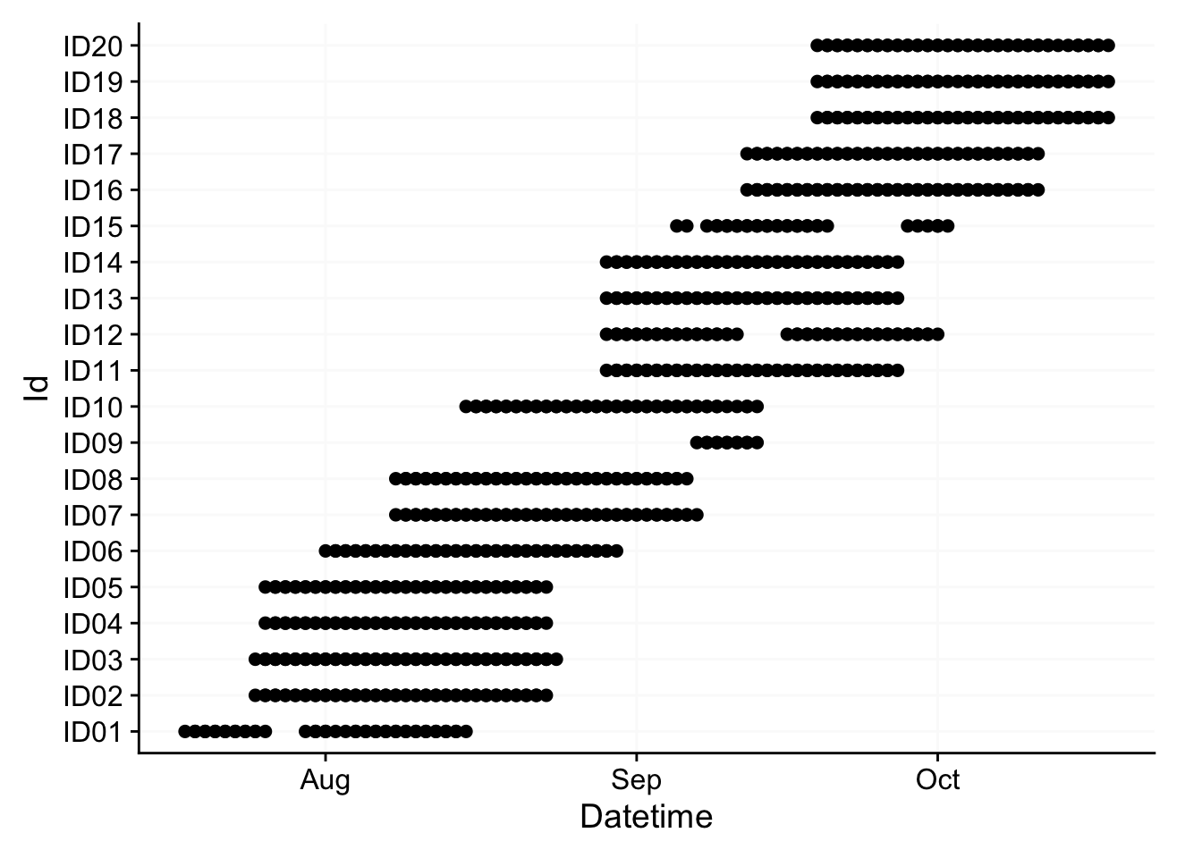
#visualize the data as a doubleplot of an average day
data_malaysia %>%
  filter(!marked_for_removal) %>%
  ungroup() %>%
  aggregate_Date(numeric.handler = \(x) mean(x, na.rm = TRUE)) %>%
  gg_doubleplot(fill = pal_jco()(1))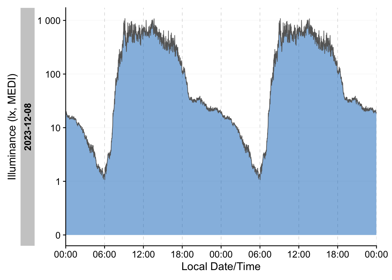
#visualize the data as a doubleplot of an average day
data_switzerland %>%
  filter(!marked_for_removal) %>%
  ungroup() %>%
  aggregate_Date(numeric.handler = \(x) mean(x, na.rm = TRUE)) %>%
  gg_doubleplot()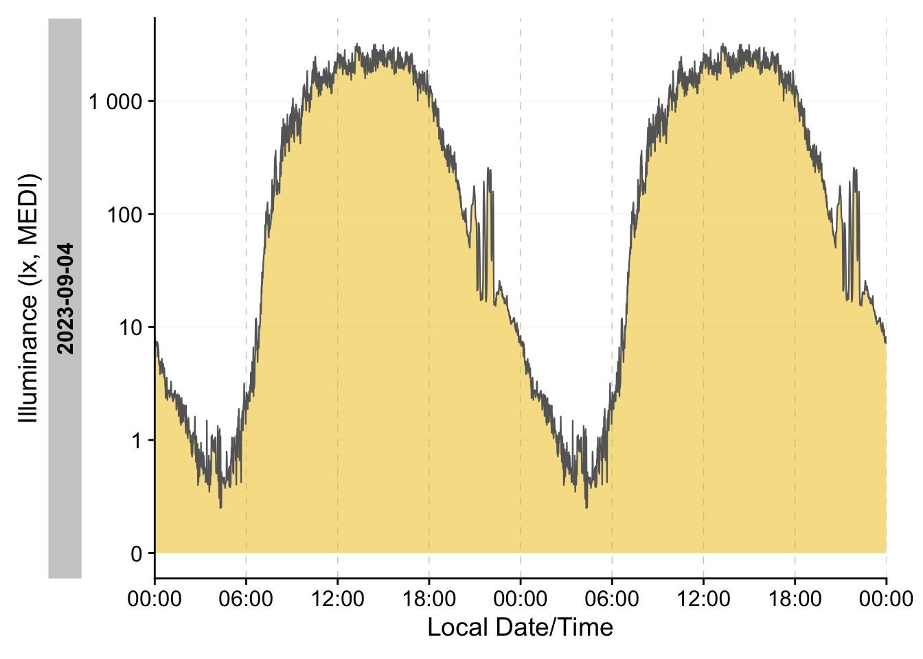
# ggsave("figures/average_day_basel.pdf", height = 27)### Combine datasets and descriptives
The datasets are combined into one dataset for further analysis.
#combine the light exposure data
data <- list(malaysia = data_malaysia %>% filter(!marked_for_removal),
             switzerland = data_switzerland %>% filter(!marked_for_removal))

descriptive <-
data %>% map(\(x) {
  x %>% tbl_summary(include = c(MEDI),
                              by = Id,
                              missing_text = "Missing",
                              statistic = list(
                                               MEDI ~ "{mean} ({min}, {max})")
                              )
})

descriptive[[1]]| Characteristic | MY001 N = 41,7601 |
MY002 N = 20,1601 |
MY003 N = 41,7601 |
MY004 N = 41,7601 |
MY005 N = 41,7601 |
MY007 N = 41,7601 |
MY008 N = 41,7601 |
MY009 N = 41,7601 |
MY010 N = 34,5601 |
MY011 N = 40,3201 |
MY012 N = 43,2001 |
MY013 N = 41,7601 |
MY014 N = 41,7601 |
MY015 N = 41,7601 |
MY016 N = 31,6801 |
MY017 N = 43,2001 |
MY018 N = 15,8401 |
MY019 N = 43,2001 |
MY020 N = 15,8401 |
|---|---|---|---|---|---|---|---|---|---|---|---|---|---|---|---|---|---|---|---|
| MEDI | 266 (0, 102,316) | 124 (0, 49,984) | 183 (0, 102,319) | 246 (0, 77,476) | 207 (0, 104,484) | 224 (0, 67,146) | 148 (0, 101,702) | 512 (0, 109,127) | 176 (0, 79,192) | 68 (0, 50,185) | 127 (0, 58,776) | 289 (0, 116,735) | 440 (0, 125,709) | 134 (0, 34,199) | 188 (0, 67,580) | 159 (0, 89,517) | 175 (0, 62,551) | 138 (0, 109,826) | 97 (0, 81,403) |
| Missing | 0 | 187 | 0 | 0 | 0 | 0 | 0 | 0 | 114 | 196 | 0 | 25 | 1 | 0 | 57 | 13 | 514 | 370 | 0 |
| 1 Mean (Min, Max) | |||||||||||||||||||
descriptive[[2]]| Characteristic | ID01 N = 33,1201 |
ID02 N = 41,7601 |
ID03 N = 41,7601 |
ID04 N = 40,3201 |
ID05 N = 40,3201 |
ID06 N = 41,7601 |
ID07 N = 43,2001 |
ID08 N = 41,7601 |
ID09 N = 8,6401 |
ID10 N = 40,3201 |
ID11 N = 41,7601 |
ID12 N = 40,3201 |
ID13 N = 41,7601 |
ID14 N = 41,7601 |
ID15 N = 23,0401 |
ID16 N = 41,7601 |
ID17 N = 41,7601 |
ID18 N = 41,7601 |
ID19 N = 40,3201 |
ID20 N = 40,3201 |
|---|---|---|---|---|---|---|---|---|---|---|---|---|---|---|---|---|---|---|---|---|
| MEDI | 1,294 (0, 130,038) | 1,005 (0, 113,549) | 1,357 (0, 125,807) | 1,337 (0, 114,184) | 425 (0, 93,199) | 804 (0, 130,088) | 1,211 (0, 114,327) | 1,047 (0, 119,789) | 79 (0, 72,266) | 306 (0, 97,892) | 1,043 (0, 120,756) | 835 (0, 105,709) | 1,134 (0, 108,602) | 548 (0, 123,006) | 187 (0, 112,956) | 481 (0, 107,579) | 311 (0, 119,461) | 1,007 (0, 117,245) | 403 (0, 117,124) | 77 (0, 93,858) |
| Missing | 375 | 25 | 228 | 21 | 23 | 129 | 22 | 25 | 0 | 21 | 51 | 0 | 25 | 26 | 322 | 26 | 29 | 36 | 485 | 34 |
| 1 Mean (Min, Max) | ||||||||||||||||||||
#combine the leba data
leba_data <- list(malaysia = leba_malaysia, switzerland = leba_switzerland)
leba_data_combined <- leba_data %>% list_rbind(names_to = "site")
var_label(leba_data_combined) <- leba_questions %>% as.list()

#histogram summary
leba_data_combined %>%
  pivot_longer(cols = -c(site, Id, Day, Datetime),
               names_to = "item", values_to = "value") %>%
  group_by(site, item) %>%
  nest() %>%
  ungroup() %>%
  mutate(question = rep(leba_questions, 2)) %>%
  unnest_wider(data) %>%
  select(-c(Id,Day, Datetime)) %>%
  mutate(value = map(value, \(x) x %>% as.numeric() %>% hist(breaks = (0.5+0:5), plot = FALSE) %>% .$counts)) %>%
  pivot_wider(id_cols = c(question, item), names_from = site, values_from = value) %>%
  gt() %>%
  cols_nanoplot(new_col_name = "Malaysia",
                columns = c(malaysia), plot_type = "bar",
                options = nanoplot_options(
                  data_bar_fill_color = pal_jco()(1),
                  data_bar_stroke_color = pal_jco()(1)
                )) %>%
  cols_nanoplot(new_col_name = "Switzerland",
                columns = c(switzerland), plot_type = "bar",
                options = nanoplot_options(
                  data_bar_fill_color = pal_jco()(2)[2],
                  data_bar_stroke_color = pal_jco()(2)[2]
                )) %>%
  cols_label(question = "LEBA Item",
item = "Item coding")| LEBA Item | Item coding | Malaysia | Switzerland |
|---|---|---|---|
| I wear blue-filtering, orange-tinted, and/or red-tinted glasses indoors during the day | leba_F1_01 | ||
| I wear blue-filtering, orange-tinted, and/or red-tinted glasses outdoors during the day | leba_F1_02 | ||
| I wear blue-filtering, orange-tinted, and/or red-tinted glasses within 1 hour before attempting to fall asleep | leba_F1_03 | ||
| I spend 30 minutes or less per day (in total) outside | leba_F2_04 | ||
| I spend between 30 minutes and 1 hour per day (in total) outside | leba_F2_05 | ||
| I spend between 1 and 3 hours per day (in total) outside | leba_F2_06 | ||
| I spend more than 3 hours per day (in total) outside | leba_F2_07 | ||
| I spend as much time outside as possible | leba_F2_08 | ||
| I go for a walk or exercise outside within 2 hours after waking up | leba_F2_09 | ||
| I use my mobile phone within 1 hour before attempting to fall asleep | leba_F3_10 | ||
| I look at my mobile phone screen immediately after waking up | leba_F3_11 | ||
| I check my phone when I wake up at night | leba_F3_12 | ||
| I look at my smartwatch within 1 hour before attempting to fall asleep | leba_F3_13 | ||
| I look at my smartwatch when I wake up at night | leba_F3_14 | ||
| I dim my mobile phone screen within 1 hour before attempting to fall asleep | leba_F4_15 | ||
| I use a blue-filter app on my computer screen within 1 hour before attempting to fall asleep | leba_F4_16 | ||
| I use as little light as possible when I get up during the night | leba_F4_17 | ||
| I dim my computer screen within 1 hour before attempting to fall asleep | leba_F4_18 | ||
| I use tunable lights to create a healthy light environment | leba_F5_19 | ||
| I use LEDs to create a healthy light environment | leba_F5_20 | ||
| I use a desk lamp when I do focused work | leba_F5_21 | ||
| I use an alarm with a dawn simulation light | leba_F5_22 | ||
| I turn on the lights immediately after waking up | leba_F5_23 |
#numeric summary plot
leba_data_combined %>%
tbl_summary(include = -c(Id, Day, Datetime), by = site)| Characteristic | malaysia N = 1711 |
switzerland N = 1751 |
|---|---|---|
| I wear blue-filtering, orange-tinted, and/or red-tinted glasses indoors during the day | ||
| Never | 128 (75%) | 150 (86%) |
| Rarely | 13 (7.6%) | 7 (4.0%) |
| Sometimes | 10 (5.8%) | 8 (4.6%) |
| Often | 11 (6.4%) | 1 (0.6%) |
| Always | 9 (5.3%) | 9 (5.1%) |
| I wear blue-filtering, orange-tinted, and/or red-tinted glasses outdoors during the day | ||
| Never | 114 (67%) | 149 (85%) |
| Rarely | 32 (19%) | 8 (4.6%) |
| Sometimes | 7 (4.1%) | 4 (2.3%) |
| Often | 10 (5.8%) | 1 (0.6%) |
| Always | 8 (4.7%) | 13 (7.4%) |
| I wear blue-filtering, orange-tinted, and/or red-tinted glasses within 1 hour before attempting to fall asleep | ||
| Never | 135 (79%) | 154 (88%) |
| Rarely | 18 (11%) | 3 (1.7%) |
| Sometimes | 7 (4.1%) | 15 (8.6%) |
| Often | 2 (1.2%) | 2 (1.1%) |
| Always | 9 (5.3%) | 1 (0.6%) |
| I spend 30 minutes or less per day (in total) outside | ||
| Never | 26 (15%) | 56 (32%) |
| Rarely | 52 (30%) | 51 (29%) |
| Sometimes | 45 (26%) | 33 (19%) |
| Often | 34 (20%) | 22 (13%) |
| Always | 14 (8.2%) | 13 (7.4%) |
| I spend between 30 minutes and 1 hour per day (in total) outside | ||
| Never | 5 (2.9%) | 22 (13%) |
| Rarely | 42 (25%) | 49 (28%) |
| Sometimes | 71 (42%) | 38 (22%) |
| Often | 39 (23%) | 47 (27%) |
| Always | 14 (8.2%) | 19 (11%) |
| I spend between 1 and 3 hours per day (in total) outside | ||
| Never | 12 (7.0%) | 38 (22%) |
| Rarely | 31 (18%) | 39 (22%) |
| Sometimes | 71 (42%) | 41 (23%) |
| Often | 46 (27%) | 43 (25%) |
| Always | 11 (6.4%) | 14 (8.0%) |
| I spend more than 3 hours per day (in total) outside | ||
| Never | 32 (19%) | 57 (33%) |
| Rarely | 45 (26%) | 46 (26%) |
| Sometimes | 41 (24%) | 38 (22%) |
| Often | 46 (27%) | 25 (14%) |
| Always | 7 (4.1%) | 9 (5.1%) |
| I spend as much time outside as possible | ||
| Never | 50 (29%) | 40 (23%) |
| Rarely | 55 (32%) | 44 (25%) |
| Sometimes | 36 (21%) | 33 (19%) |
| Often | 25 (15%) | 34 (19%) |
| Always | 5 (2.9%) | 24 (14%) |
| I go for a walk or exercise outside within 2 hours after waking up | ||
| Never | 103 (60%) | 71 (41%) |
| Rarely | 50 (29%) | 53 (30%) |
| Sometimes | 13 (7.6%) | 27 (15%) |
| Often | 5 (2.9%) | 19 (11%) |
| Always | 0 (0%) | 5 (2.9%) |
| I use my mobile phone within 1 hour before attempting to fall asleep | ||
| Never | 6 (3.5%) | 1 (0.6%) |
| Rarely | 1 (0.6%) | 9 (5.1%) |
| Sometimes | 4 (2.3%) | 13 (7.4%) |
| Often | 37 (22%) | 41 (23%) |
| Always | 123 (72%) | 111 (63%) |
| I look at my mobile phone screen immediately after waking up | ||
| Never | 9 (5.3%) | 7 (4.0%) |
| Rarely | 20 (12%) | 16 (9.1%) |
| Sometimes | 31 (18%) | 25 (14%) |
| Often | 42 (25%) | 57 (33%) |
| Always | 69 (40%) | 70 (40%) |
| I check my phone when I wake up at night | ||
| Never | 27 (16%) | 80 (46%) |
| Rarely | 32 (19%) | 38 (22%) |
| Sometimes | 53 (31%) | 25 (14%) |
| Often | 23 (13%) | 14 (8.0%) |
| Always | 36 (21%) | 18 (10%) |
| I look at my smartwatch within 1 hour before attempting to fall asleep | ||
| Never | 148 (87%) | 154 (88%) |
| Rarely | 22 (13%) | 1 (0.6%) |
| Sometimes | 1 (0.6%) | 6 (3.4%) |
| Often | 0 (0%) | 9 (5.1%) |
| Always | 0 (0%) | 5 (2.9%) |
| I look at my smartwatch when I wake up at night | ||
| Never | 160 (94%) | 157 (90%) |
| Rarely | 11 (6.4%) | 0 (0%) |
| Sometimes | 0 (0%) | 4 (2.3%) |
| Often | 0 (0%) | 12 (6.9%) |
| Always | 0 (0%) | 2 (1.1%) |
| I dim my mobile phone screen within 1 hour before attempting to fall asleep | ||
| Never | 47 (27%) | 51 (29%) |
| Rarely | 17 (9.9%) | 20 (11%) |
| Sometimes | 33 (19%) | 22 (13%) |
| Often | 33 (19%) | 38 (22%) |
| Always | 41 (24%) | 44 (25%) |
| I use a blue-filter app on my computer screen within 1 hour before attempting to fall asleep | ||
| Never | 114 (67%) | 123 (70%) |
| Rarely | 9 (5.3%) | 2 (1.1%) |
| Sometimes | 3 (1.8%) | 8 (4.6%) |
| Often | 13 (7.6%) | 9 (5.1%) |
| Always | 32 (19%) | 33 (19%) |
| I use as little light as possible when I get up during the night | ||
| Never | 13 (7.6%) | 16 (9.1%) |
| Rarely | 18 (11%) | 12 (6.9%) |
| Sometimes | 46 (27%) | 23 (13%) |
| Often | 54 (32%) | 18 (10%) |
| Always | 40 (23%) | 106 (61%) |
| I dim my computer screen within 1 hour before attempting to fall asleep | ||
| Never | 59 (35%) | 103 (59%) |
| Rarely | 26 (15%) | 17 (9.7%) |
| Sometimes | 26 (15%) | 12 (6.9%) |
| Often | 28 (16%) | 22 (13%) |
| Always | 32 (19%) | 21 (12%) |
| I use tunable lights to create a healthy light environment | ||
| Never | 128 (75%) | 134 (77%) |
| Rarely | 15 (8.8%) | 13 (7.4%) |
| Sometimes | 22 (13%) | 10 (5.7%) |
| Often | 5 (2.9%) | 5 (2.9%) |
| Always | 1 (0.6%) | 13 (7.4%) |
| I use LEDs to create a healthy light environment | ||
| Never | 89 (52%) | 141 (81%) |
| Rarely | 19 (11%) | 12 (6.9%) |
| Sometimes | 35 (20%) | 9 (5.1%) |
| Often | 15 (8.8%) | 5 (2.9%) |
| Always | 13 (7.6%) | 8 (4.6%) |
| I use a desk lamp when I do focused work | ||
| Never | 128 (75%) | 138 (79%) |
| Rarely | 20 (12%) | 9 (5.1%) |
| Sometimes | 5 (2.9%) | 13 (7.4%) |
| Often | 13 (7.6%) | 11 (6.3%) |
| Always | 5 (2.9%) | 4 (2.3%) |
| I use an alarm with a dawn simulation light | ||
| Never | 143 (84%) | 166 (95%) |
| Rarely | 14 (8.2%) | 0 (0%) |
| Sometimes | 12 (7.0%) | 1 (0.6%) |
| Often | 2 (1.2%) | 5 (2.9%) |
| Always | 0 (0%) | 3 (1.7%) |
| I turn on the lights immediately after waking up | ||
| Never | 27 (16%) | 74 (42%) |
| Rarely | 39 (23%) | 39 (22%) |
| Sometimes | 59 (35%) | 19 (11%) |
| Often | 31 (18%) | 21 (12%) |
| Always | 15 (8.8%) | 22 (13%) |
| 1 n (%) | ||
4.2 Calculate the photoperiod
In this section, the dataset is extended by by a column indicating one of three states of the day: day, evening, and night. The states are determined by the photoperiod of the location of the data collection. day is defined as the time between sunrise (dawn) and sunset (dusk), evening as the time between sunset and the midnight, and night as the time between midnight and sunrise. Midnight is chosen as a somewhat arbitrary differentiator between states, as sleep timing is not available in the dataset or auxiliary data collection.
#extract the days for the data collection
relevant_days <-
  data %>%
  map(~ .x %>% ungroup() %>% pull(Day) %>% unique)

#calculate sunrise and sunset times for the location of the data collection
photoperiods <-
  names(data) %>%
  rlang::set_names() %>%
  map(\(x) {
        photoperiod(coordinates[[x]], relevant_days[[x]], tz = tzs[[x]])
  })

#add the photoperiod to the data
data <-
  data %>%
  map2(photoperiods, ~ left_join(.x, .y, by = c("Day" = "date")))

#set categories for the photoperiod
data <-
  data %>%
  map(\(x) {
    x %>%
      group_by(Day, .add = TRUE) %>%
      mutate(Photoperiod = case_when(
        Datetime < dawn ~ "night",
        Datetime < dusk ~ "day",
        Datetime >= dusk ~ "evening"),
        photoperiod_duration = sum(Photoperiod == "day")/60
      ) %>%
      ungroup(Day)
  })

#display an exemplary week with photoperiods

data %>%
  map2(c("MY001", "ID01"), \(x,y) {
    x %>%
  filter(!marked_for_removal) %>%
  filter(Id == y) %>%
  filter_Date(length = "1 week") %>%
  gg_day(geom = "ribbon", alpha = 0.5, col = "black", aes_fill = Id) +
  geom_rect(data = \(x) x %>% summarize(dawn = mean(hms::as_hms(dawn)),
                                         dusk = mean(hms::as_hms(dusk))),
   aes(xmin = 0, xmax = dawn, ymin = -Inf, ymax = Inf), alpha = 0.25)+
  geom_rect(data = \(x) x %>% summarize(dawn = mean(hms::as_hms(dawn)),
                                         dusk = mean(hms::as_hms(dusk))),
   aes(xmin = dusk, xmax = 24*60*60, ymin = -Inf, ymax = Inf), alpha = 0.25)+
  theme(legend.position = "none")+
  labs(title = paste0("Example week with photoperiod for participant ", y))

  })
$malaysia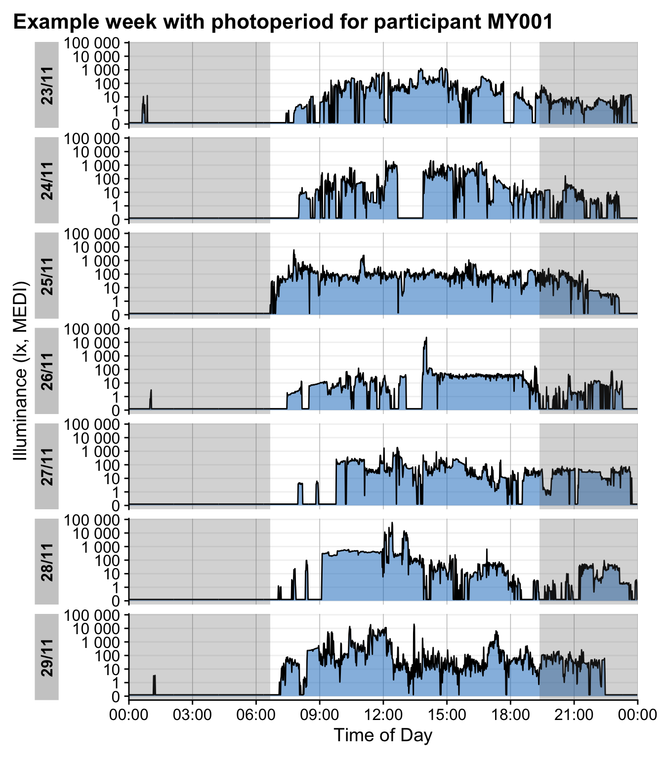
$switzerland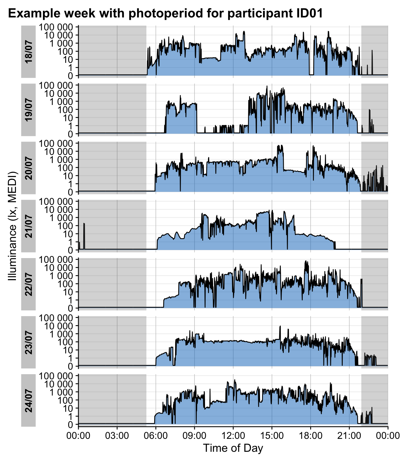
The dataset spans a period of 39 days in Malaysia and 92 days in Switzerland.
5 Inferential Analysis
5.1 Photoperiod duration
photoperiods <-
data %>% list_rbind(names_to = "site") %>%
  group_by(site, Day, photoperiod_duration) %>%
  summarize(.groups = "drop")

t.test(photoperiod_duration ~ site, data = photoperiods)
    Welch Two Sample t-test

data:  photoperiod_duration by site
t = -10.851, df = 91.007, p-value < 2.2e-16
alternative hypothesis: true difference in means between group malaysia and group switzerland is not equal to 0
95 percent confidence interval:
 -1.998324 -1.379909
sample estimates:
   mean in group malaysia mean in group switzerland
                 12.70128                  14.39040
Photoperiods are significantly different between sites. Thus applicable metrics will be corrected by duration of photoperiod (cd). In the case of evening or night data (e.g., TBTe10), correction will be done on their respective duration. This was not specified in the preregistration document.
5.2 Research Question 1
RQ 1: Are there differences in objectively measured light exposure between the two sites, and if so, in which light metrics?
5.2.1 Hypothesis 1
\(H1\): There are differences in light logger-derived light exposure intensity levels and duration of intensity between Malaysia and Switzerland.
5.2.1.1 Metric calculation
In this section, metrics will be calculated for the light exposure data.
The metrics are as follows:
H1:
Time above Threshold 250 lx mel EDI (TAT250)
Time above Threshold 1000 lx mel EDI (TAT1000)
Period above Threshold 1000 lx mel EDI (PAT1000)
Time above Threshold 250 lx mel EDI during daytime hours (TATd250)
Time below Threshold 10 lx mel EDI during evening hours (TBTe10)
metric_selection <- list(
  H1 = c("TAT250", "TAT1000", "PAT1000", "TATd250", "TBTe10")
)

p_adjustment <- list(
  H1 = 5
)

metrics <-
  data %>%
  map(
    \(x) {
      #whole-day metrics
      whole_day <-
      x %>%
        group_by(Id, Day) %>%
        summarize(
          TAT250 =
            duration_above_threshold(MEDI, Datetime, "above", 250, na.rm = TRUE),
          TAT1000 =
            duration_above_threshold(MEDI, Datetime, "above", 1000, na.rm = TRUE),
          PAT1000 =
            period_above_threshold(MEDI, Datetime, "above", 1000, na.rm = TRUE),
          .groups = "drop",
          photoperiod_duration = first(photoperiod_duration)
        ) %>%
        mutate(across(where(is.duration), as.numeric)) %>%
        pivot_longer(cols = -c(Id, Day, photoperiod_duration), names_to = "metric")

      #part-day metrics
      part_day <-
        x %>%
        group_by(Id, Day, Photoperiod) %>%
        summarize(
          TATd250 =
            duration_above_threshold(MEDI, Datetime, "above", 250, na.rm = TRUE),
          TBTe10 =
            duration_above_threshold(MEDI, Datetime, "below", 10, na.rm =  TRUE),
          .groups = "drop",
          photoperiod_duration = first(photoperiod_duration)
        ) %>%
        mutate(across(where(is.duration), as.numeric)) %>%
        pivot_longer(cols = -c(Id, Day, Photoperiod,
                               photoperiod_duration), names_to = "metric") %>%
        filter((Photoperiod == "day" & metric == "TATd250") |
               (Photoperiod == "evening" & metric == "TBTe10"))

      whole_day %>%
        bind_rows(part_day)
    }
  ) %>%
  list_rbind(names_to = "site") %>%
  nest(data = -metric)
5.2.1.2 Model fitting
All models for Hypothesis 1 showed very poor model diagnostics under a gaussian error distribution. According to the parameter metrics, the poisson family is a much more appropriate error distribution.
formula_H1 <- value_dc ~ site + (1|site:Id)
formula_H0 <- value_dc ~ 1 + (1|site:Id)

map <- purrr::map

inference_H1 <-
  metrics %>%
  filter(metric %in% metric_selection$H1) %>%
  mutate(data =
           data %>%
           purrr::map(\(x) x %>% mutate(value_dc =
                                   (value/photoperiod_duration) %>% round()))
         )

inference_H1 <-
  inference_H1 %>%
  inference_summary(formula_H1, formula_H0, p_adjustment = p_adjustment$H1,
                    family = poisson())


H1_table <-
Inference_Table(inference_H1, p_adjustment = p_adjustment$H1, value = value_dc)

H1_table <-
H1_table %>%
  tab_footnote(
    "Exponentiated beta coefficients from the final model, denoting the multiplication factor for the intercept, conditional on the site",
    locations = cells_column_labels(columns = c("malaysia", "switzerland"))
  ) %>%
  tab_footnote(
    "Model prediction for the intercept per hour of photo- or nighttime period, reference level for the site is Malaysia",
    locations = cells_column_labels(columns = "Intercept")
  ) %>%
  fmt_duration(columns = Intercept, input_units = "seconds") %>%
  fmt_number("Intercept", decimals = 0) %>%
  fmt_number("switzerland", decimals = 3) %>%
  tab_header(title = "Model Results for Hypothesis 1", )

H1_table| Model Results for Hypothesis 1 | |||||
|---|---|---|---|---|---|
| p-value1 | Intercept2 |
Site coefficients
|
|||
| Malaysia3 | Switzerland3 | ||||
| TAT250 | 0.002 | 418 | 1 | 1.780 |  |
| TAT1000 | 0.011 | 180 | 1 | 1.942 |  |
| PAT1000 | 0.15 | 78 | — | — |  |
| TATd250 | 0.003 | 410 | 1 | 1.772 |  |
| TBTe10 | 0.9
|
678 | — | — |  |
| 1 p-values are adjusted for multiple comparisons using the false-discovery-rate for n= 5 comparisons | |||||
| 2 Model prediction for the intercept per hour of photo- or nighttime period, reference level for the site is Malaysia | |||||
| 3 Exponentiated beta coefficients from the final model, denoting the multiplication factor for the intercept, conditional on the site | |||||
v1 <- gt::extract_cells(H1_table, switzerland, 1) %>% as.numeric() %>% round(3)
v2 <- gt::extract_cells(H1_table, switzerland, 2) %>% as.numeric() %>% round(3)
v3 <- gt::extract_cells(H1_table, switzerland, 4) %>% as.numeric() %>% round(3)
The model summary shows that swiss participants have significantly more time above threshold for 250 (TAT250) and 1000 lx (TAT1000) than participants in Malaysia, i.e., x1.78 and x1.942, respectively (x1.772 over 250 lx mel EDI during daytime hours, TATd250).
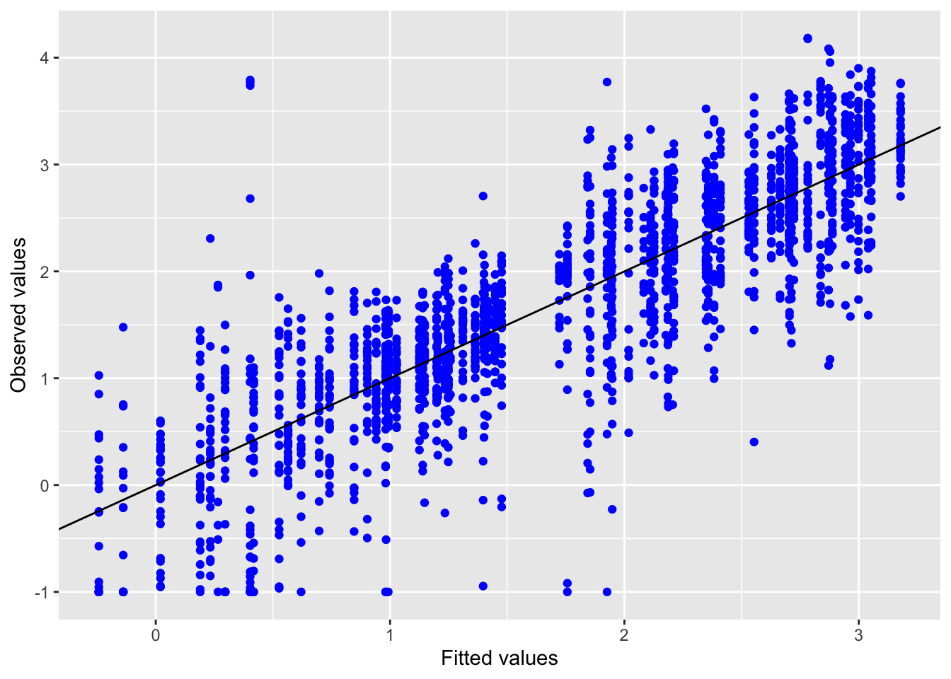
5.2.1.3 Model diagnostics
Inf_plots1(x, z)
Inf_plots2(x, z)
Inf_plots3(x, z, value_dc, "exp")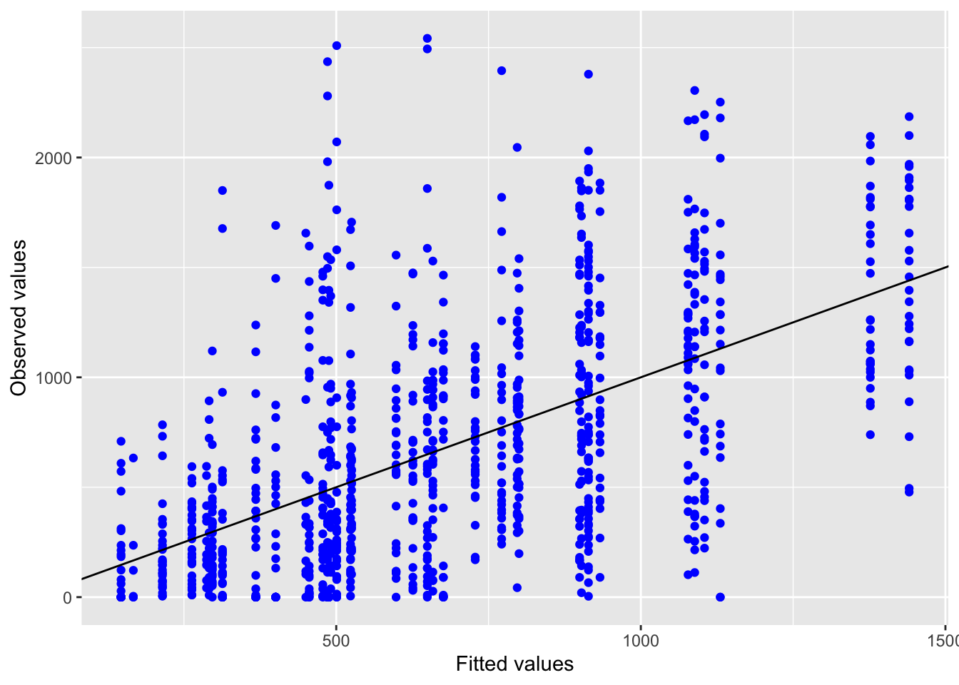
Inf_plots1(x, z)
Inf_plots2(x, z)
Inf_plots3(x, z, value_dc, "exp")
Inf_plots1(x, z)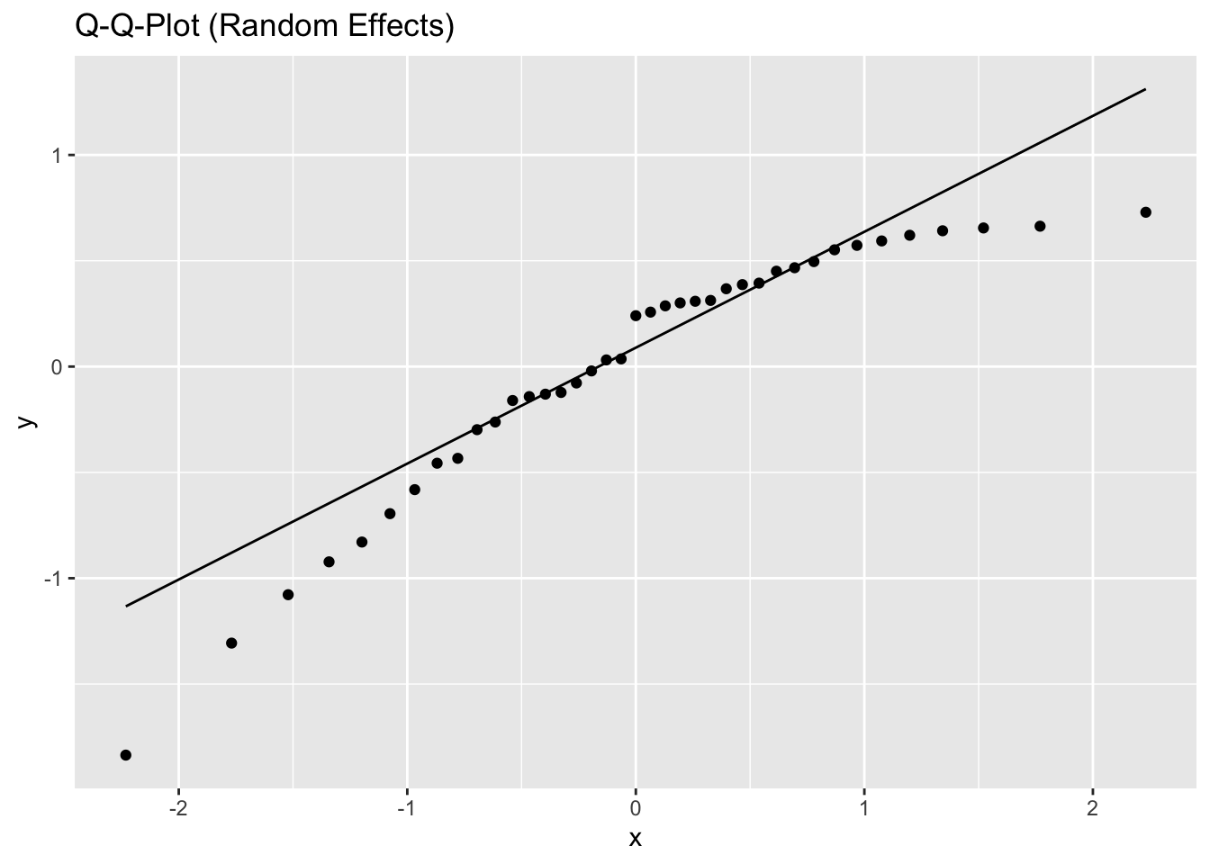
Inf_plots2(x, z)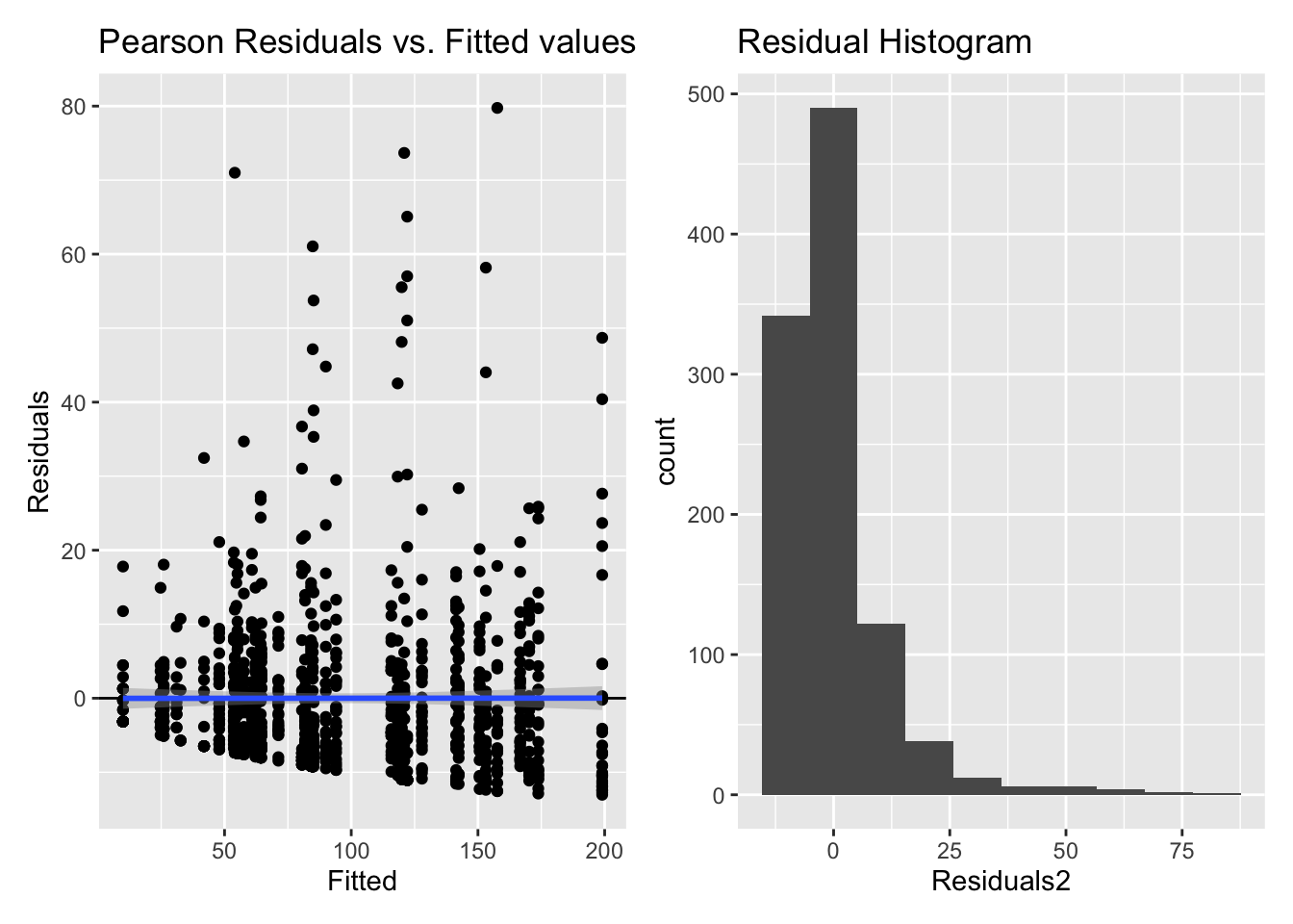
Inf_plots3(x, z, value_dc, "exp")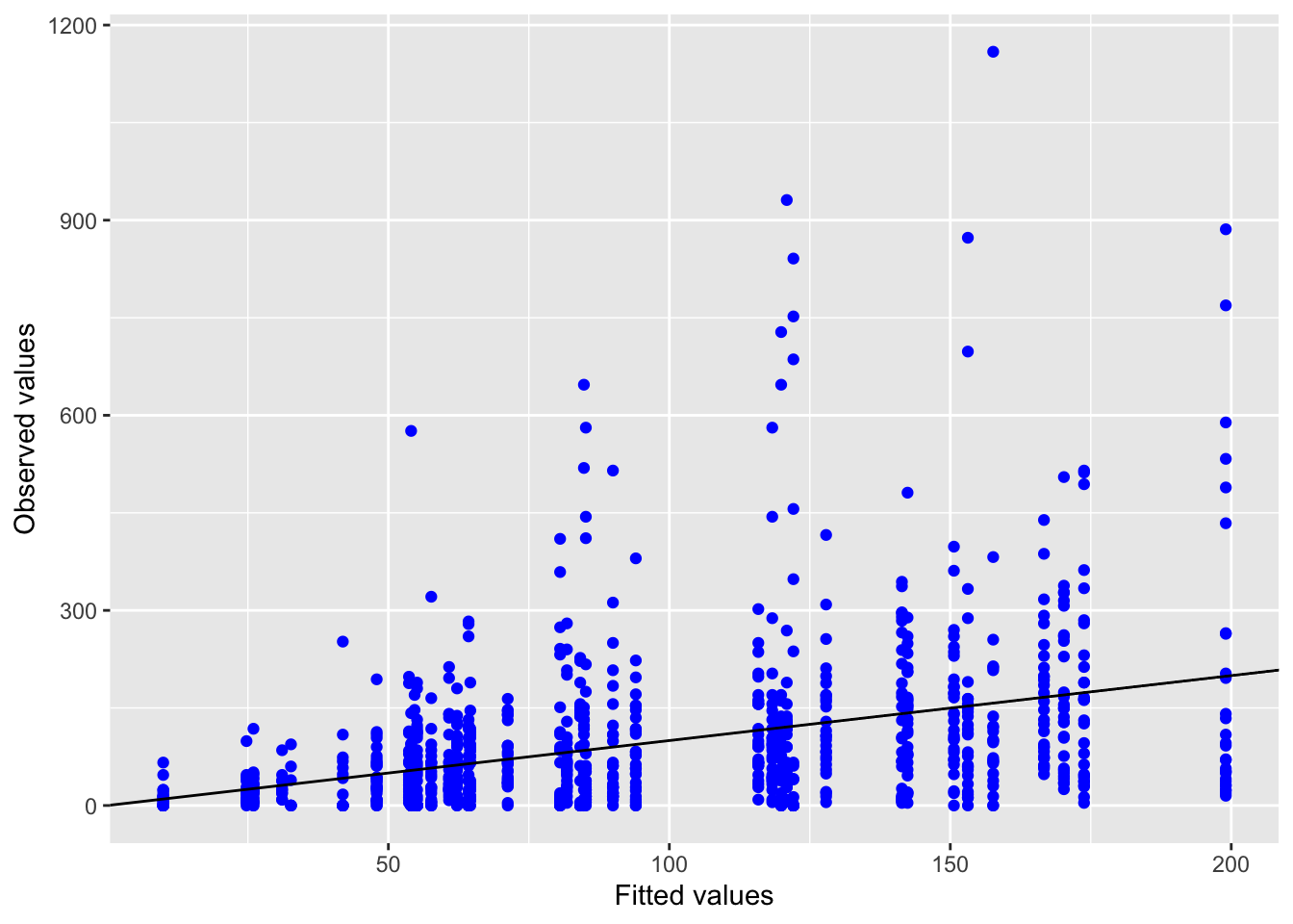
Inf_plots1(x, z)
Inf_plots2(x, z)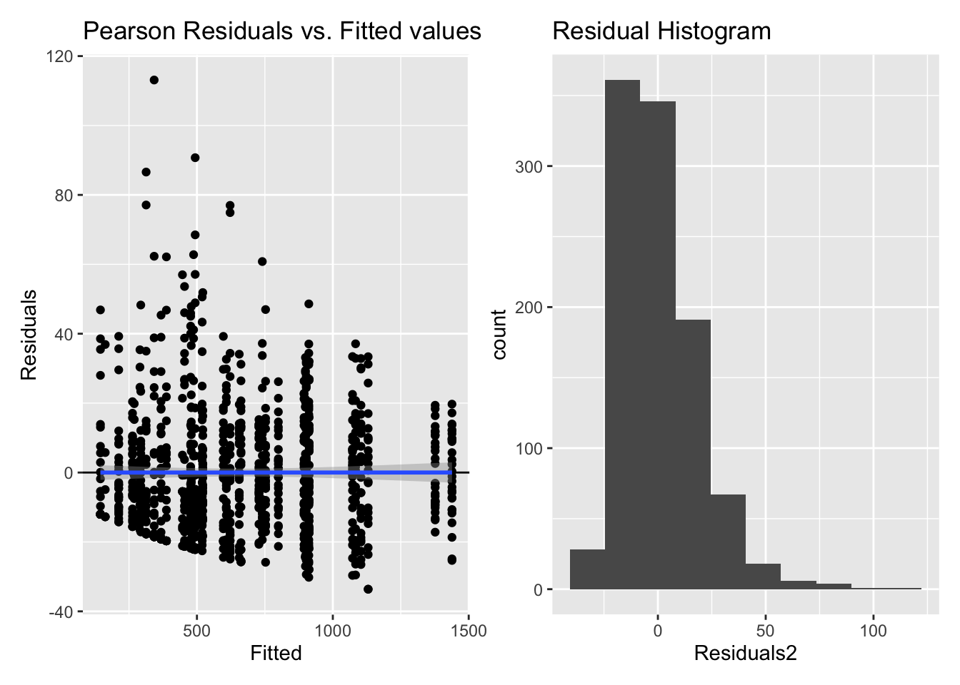
Inf_plots3(x, z, value_dc, "exp")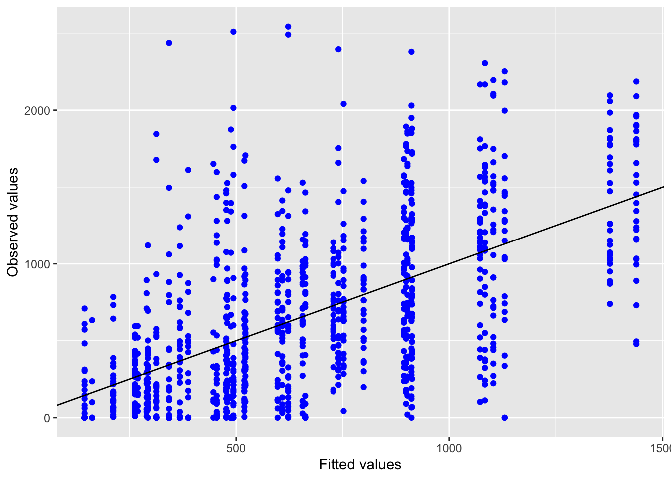
Inf_plots1(x, z)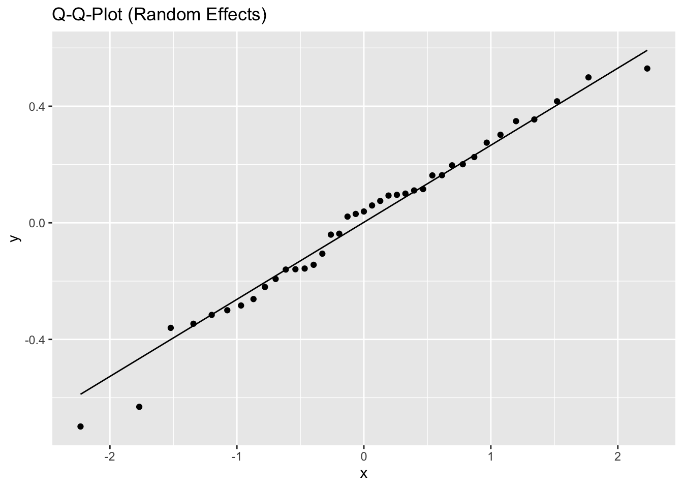
Inf_plots2(x, z)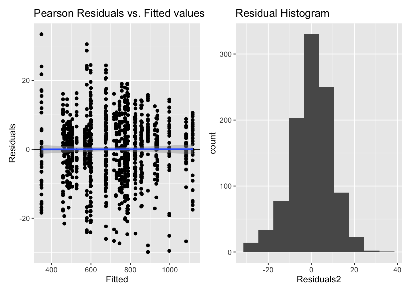
Inf_plots3(x, z, value_dc, "exp")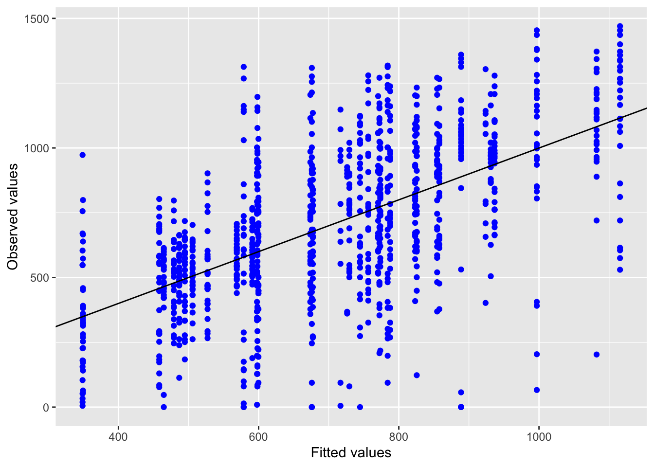
5.2.2 Hypothesis 2
\(H2\): There are differences in light logger-derived timing of light exposure between Malaysia and Switzerland.
5.2.2.1 Metric calculation
H2:
M10m
L5m
IS
IV
LLiT 10
LLiT 250
Frequency crossing Threshold 250
mean logarithmic melanopic EDI day & night
metric_selection <- append(metric_selection, list(
    H2_timing = c("M10m", "L5m", "IS", "IV", "LLiT10", "LLiT250", "FcT250"),
  H2_interaction = "mean"
)
)

p_adjustment <- append(
  p_adjustment,
  list(
  H2 = 9
))

metrics <-
  rbind(
    metrics,
      data %>%
  map(
    \(x) {
      #whole-day metrics
      whole_day <-
      x %>%
        group_by(Id, Day) %>%
        summarize(
          .groups = "drop",
          M10m =
            bright_dark_period(
                  MEDI, Datetime, "brightest", "10 hours",
                  as.df = TRUE, na.rm = TRUE
                  ) %>% pull(brightest_10h_mean) %>% log10(),
          L5m =
            bright_dark_period(
                  MEDI, Datetime, "darkest", "5 hours", as.df = TRUE,
                  loop = TRUE, na.rm = TRUE
                  ) %>% pull(darkest_5h_mean) %>% log10(),
          IV = intradaily_variability(MEDI, Datetime),
          LLiT10 =
            timing_above_threshold(
              MEDI, Datetime, "above", 10, as.df = TRUE) %>%
            pull(last_timing_above_10) %>% hms::as_hms() %>% as.numeric(),
          LLiT250 =
            timing_above_threshold(MEDI, Datetime, "above", 250, as.df = TRUE) %>%
            pull(last_timing_above_250) %>% hms::as_hms() %>% as.numeric(),
          FcT250 =
            frequency_crossing_threshold(MEDI, 250, na.rm = TRUE),
        ) %>%
        mutate(across(where(is.duration), as.numeric)) %>%
        pivot_longer(cols = -c(Id, Day), names_to = "metric")

      #part-day metrics
      part_day <-
        x %>%
        group_by(Id, Day, Photoperiod) %>%
        summarize(
          .groups = "drop",
          mean = mean(MEDI, na.rm = TRUE) %>% log10()
        ) %>%
        pivot_longer(cols = -c(Id, Day, Photoperiod), names_to = "metric") %>%
        filter(Photoperiod != "night" & metric == "mean")

      #no-day metrics
      no_day <-
          x %>%
        summarize(IS = interdaily_stability(MEDI, Datetime, na.rm = TRUE)) %>%
        pivot_longer(cols = IS, names_to = "metric")

      whole_day %>%
        bind_rows(part_day, no_day)
    }
  ) %>%
  list_rbind(names_to = "site") %>%
  nest(data = -metric)
  )
Hypothesis 2 is analyzed in three distinct ways. The first part is similar to hypothesis 1 but looks at different metrics, that are associated with the timing of light (Timing). The second part looks at the possible interaction of light during the day to the evening (Interaction). And the third part looks at a model of light across the whole day as a smooth pattern (Pattern).
5.2.2.2 Timing
formula_H2_timing <- value ~ site + (1|site:Id)
formula_H2_IV <- value ~ site
formula_H0 <- value ~ 1 + (1|site:Id)
formula_H0_IV <- value ~ 1

lmer <- lme4::lmer

inference_H2 <-
  metrics %>%
  filter(metric %in% metric_selection$H2_timing) %>%
  mutate(formula_H1 = case_match(metric,
                                 "IS" ~ c(formula_H2_IV),
                                 .default = c(formula_H2_timing)),
         formula_H0 = case_match(metric,
                                 "IS" ~ c(formula_H0_IV),
                                 .default = c(formula_H0)),
         type = (case_match(metric,
                                 "IS" ~ "lm",
                                 .default = "lmer")),
         family = list(gaussian())
         )


inference_H2 <-
  inference_H2 %>%
  inference_summary2(p_adjustment = p_adjustment$H2)

H2_table_timing <-
Inference_Table(inference_H2, p_adjustment = p_adjustment$H2, value = value) %>%
  fmt_number("Intercept", decimals = 2) %>%
  fmt_number("switzerland", decimals = 2) %>%
  cols_align(align = "center", columns = "p.value") %>%
  tab_header(title = "Model Results for Hypothesis 2, Timing", ) %>%
  fmt_duration(columns = c(Intercept, switzerland),
               input_units = "seconds",
               rows = 4:5, duration_style = "colon-sep") %>%
  tab_footnote(
    "Values were log10 transformed before model fitting",
    locations = cells_stub(rows = 1:2)
  )

H2_table_timing| Model Results for Hypothesis 2, Timing | |||||
|---|---|---|---|---|---|
| p-value1 | Intercept |
Site coefficients
|
|||
| Malaysia | Switzerland | ||||
| M10m2 | 0.004 | 2.36 | 0 | 0.46 |  |
| L5m2 | 0.2 | −0.88 | — | — |  |
| IV | 0.9
|
1.34 | — | — |  |
| LLiT10 | 0.005 | 23:16:14 | 0 | −01:10:42 |  |
| LLiT250 | <0.001 | 17:41:23 | 0 | 01:27:54 |  |
| FcT250 | 0.005 | 35.79 | 0 | 28.71 |  |
| IS | 0.9
|
0.16 | — | — |  |
| 1 p-values are adjusted for multiple comparisons using the false-discovery-rate for n= 9 comparisons | |||||
| 2 Values were log10 transformed before model fitting | |||||
v1 <-  gt::extract_cells(H2_table_timing, Intercept, 1) %>% as.numeric()
v2 <-  gt::extract_cells(H2_table_timing, switzerland, 1) %>% as.numeric()
v3 <-  gt::extract_cells(H2_table_timing, switzerland, 4)
v4 <-  gt::extract_cells(H2_table_timing, switzerland, 5)
v5 <-  gt::extract_cells(H2_table_timing, switzerland, 6) %>% as.numeric()
v6 <-  gt::extract_cells(H2_table_timing, Intercept, 6) %>% as.numeric()
The model summary shows that the 10 brightest hours (M10m) of swiss participants are significantly brighter than for participants in Malaysia, i.e., an average of 661 lx and 229 lx, respectively and the frequency of crossing 250 lx is about 2 times as high for swiss participants compared to malaysian participants (64 compared to 36, respectively). Swiss participants last time above 250 lx melanopic EDI (LLiT250) is about 1.5 hours later compared to malaysian participants (+01:27:54), and swiss participants avoid values above 10 lx after sundown (LLiT10) about 1 hour earlier compared to malaysia (−01:10:42).
5.2.2.2.1 Model diagnostics
Inf_plots1(x, z)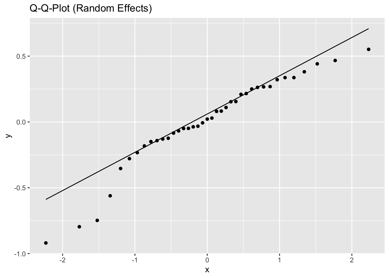
Inf_plots2(x, z)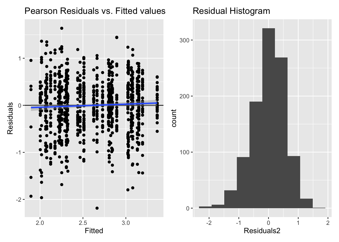
Inf_plots3(x, z %>% drop_na(value), value, transformation = "identity")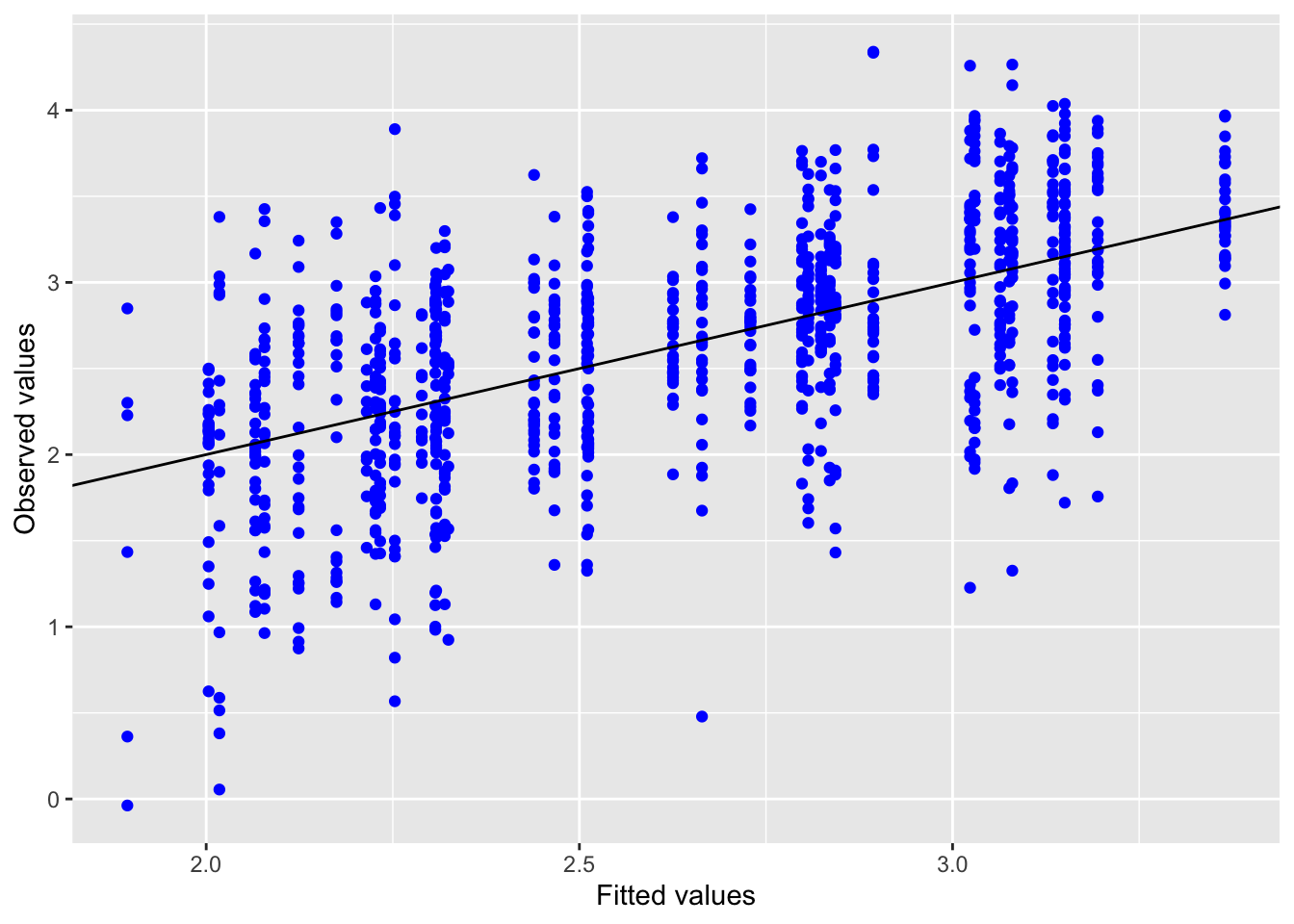
Inf_plots1(x, z)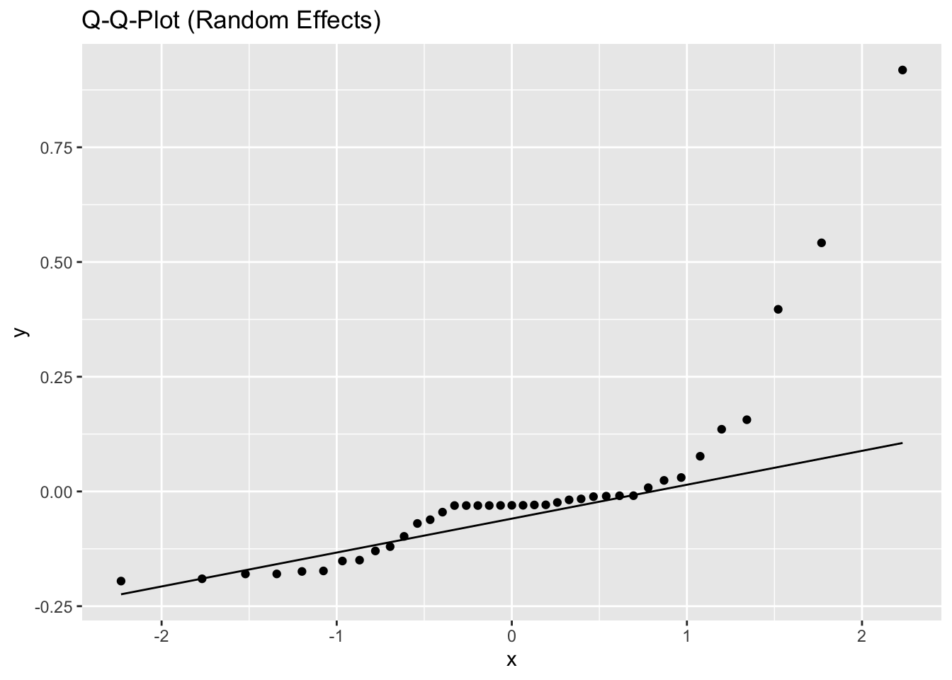
Inf_plots2(x, z)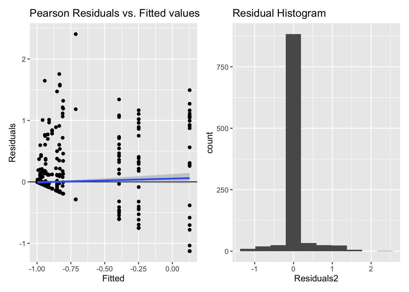
Inf_plots3(x, z %>% drop_na(value), value, transformation = "identity")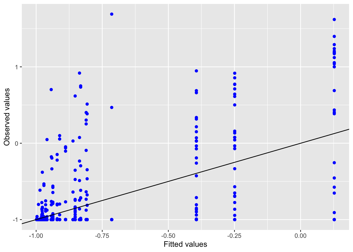
Inf_plots1(x, z)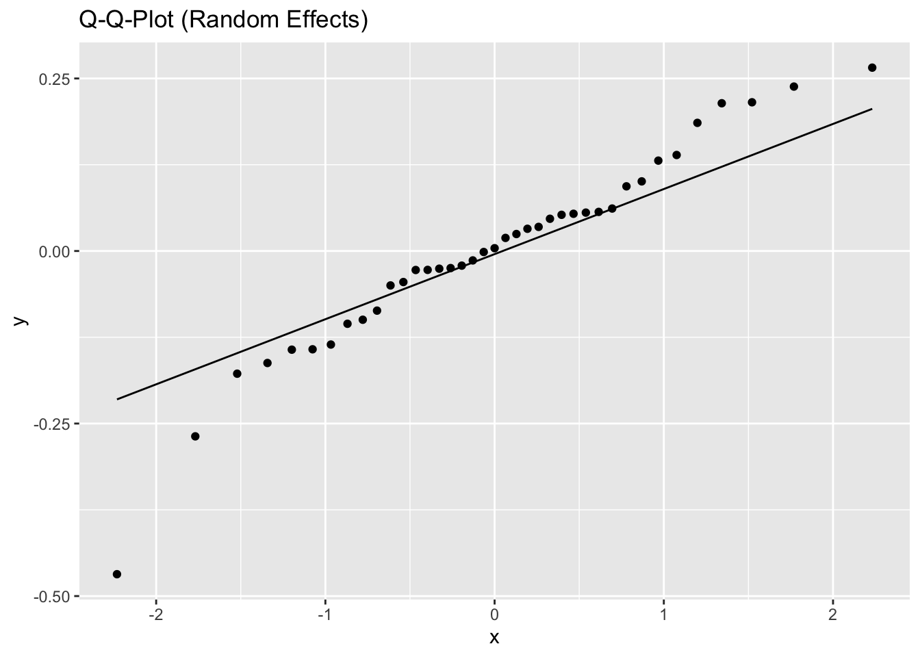
Inf_plots2(x, z)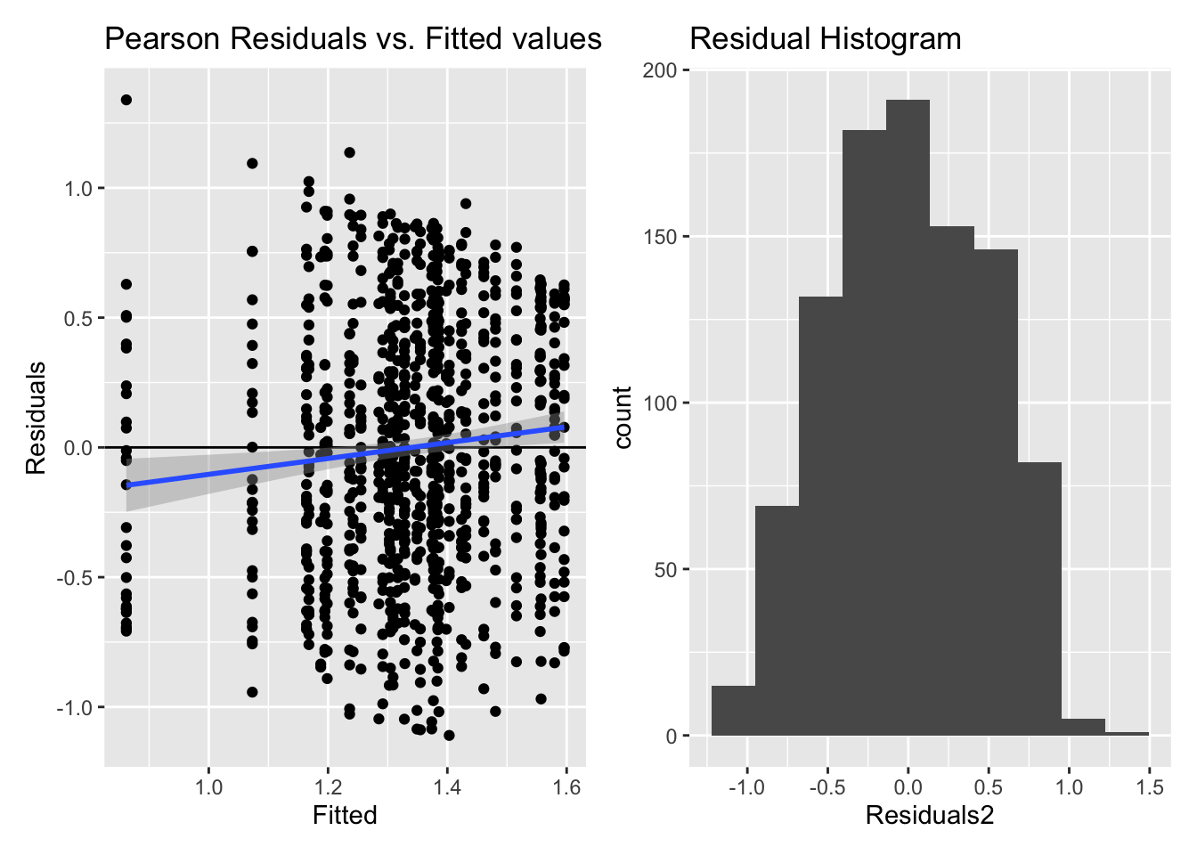
Inf_plots3(x, z %>% drop_na(value), value, transformation = "identity")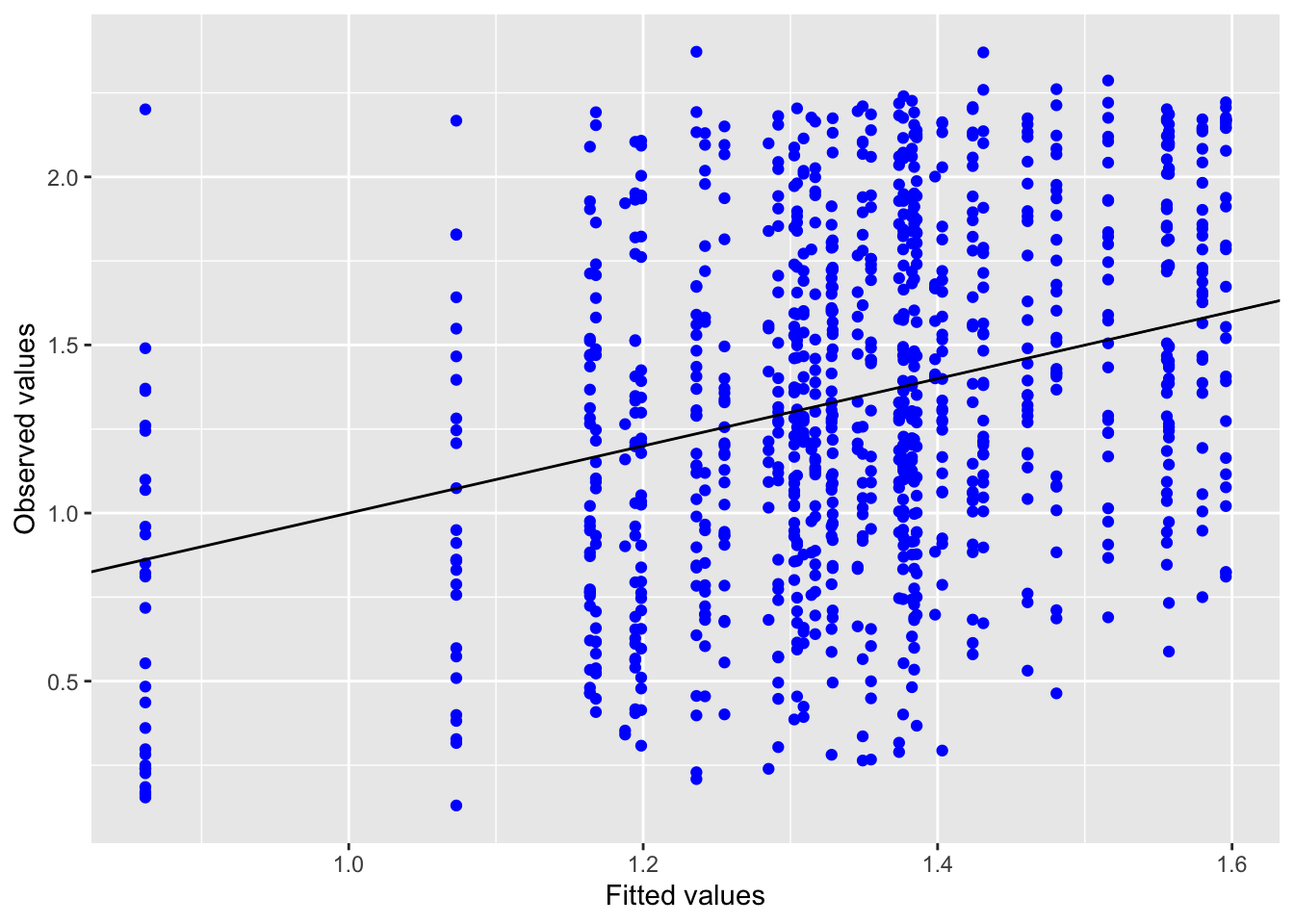
Inf_plots1(x, z)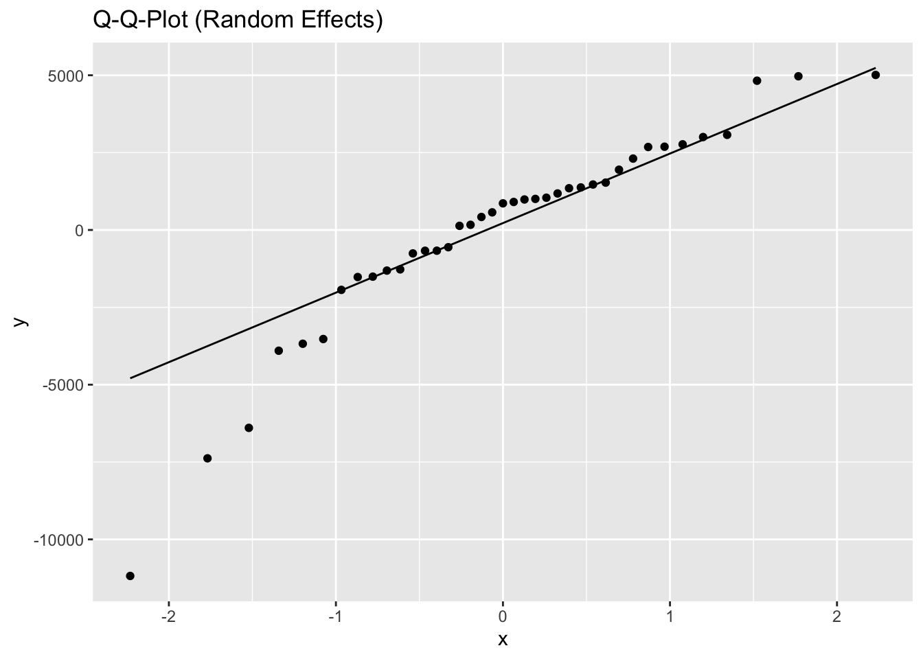
Inf_plots2(x, z)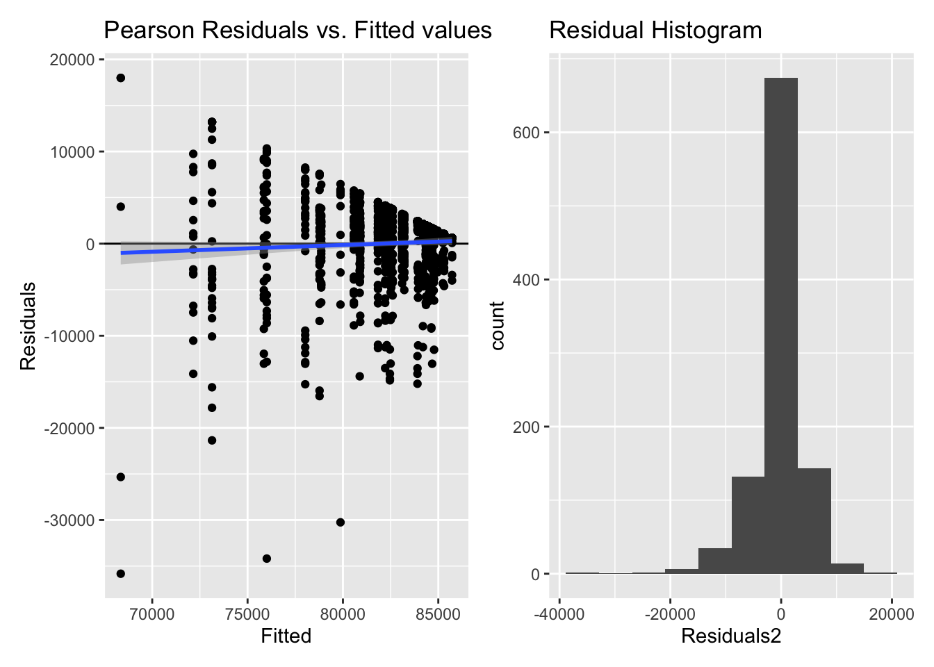
Inf_plots3(x, z %>% drop_na(value), value, transformation = "identity")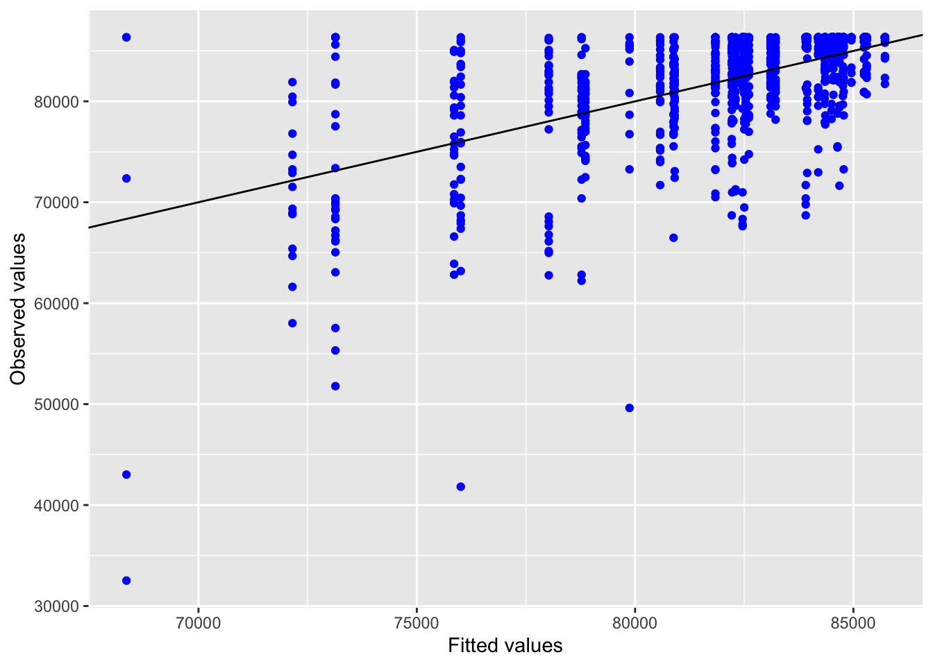
Inf_plots1(x, z)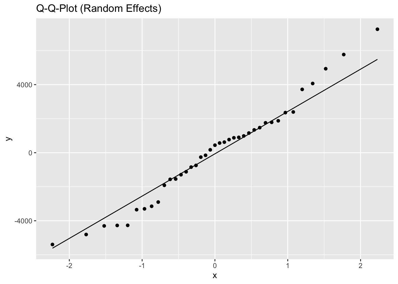
Inf_plots2(x, z)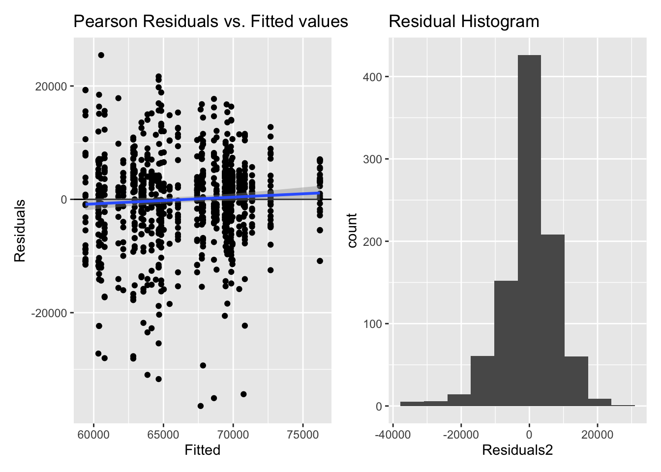
Inf_plots3(x, z %>% drop_na(value), value, transformation = "identity")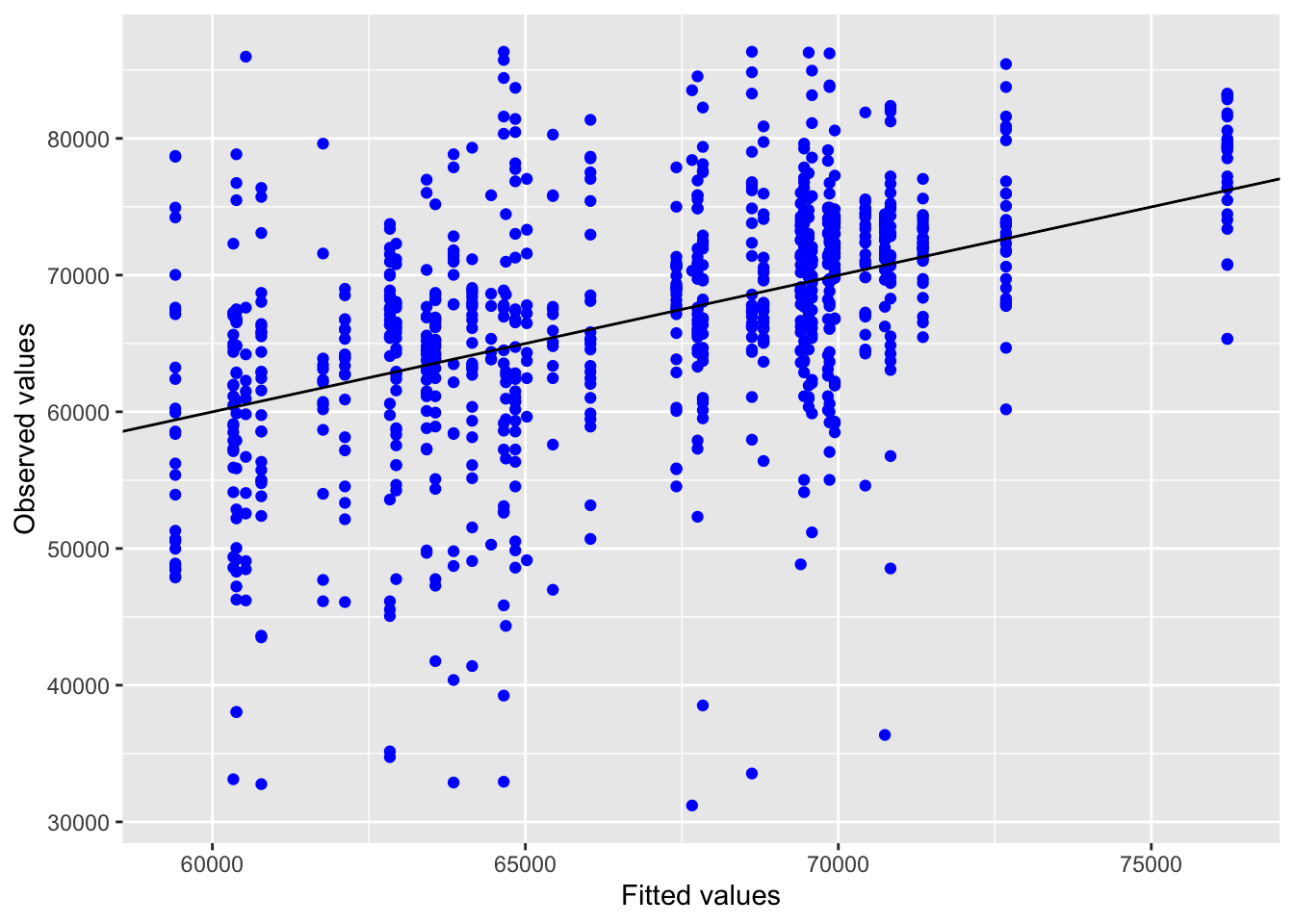
Inf_plots1(x, z)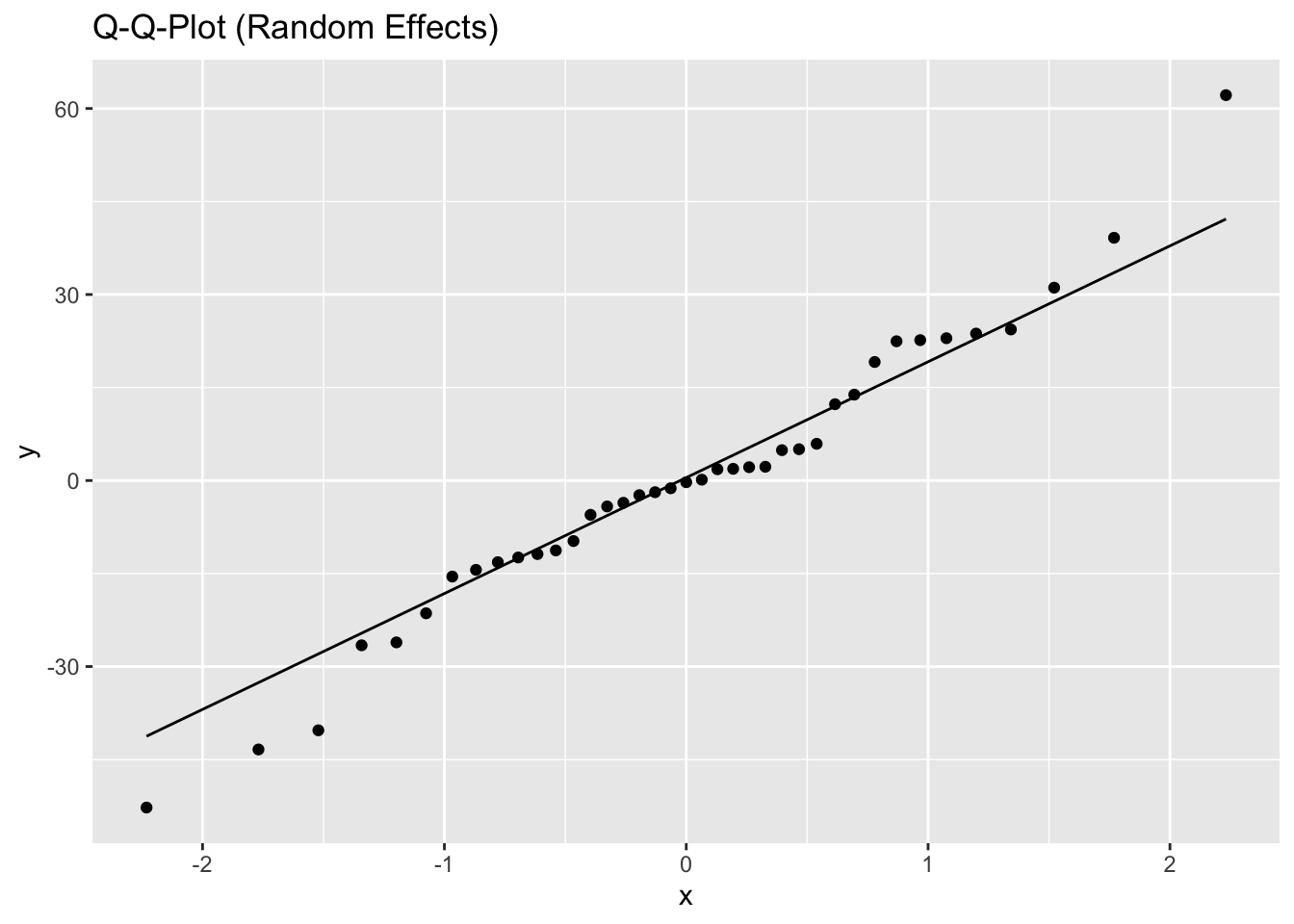
Inf_plots2(x, z)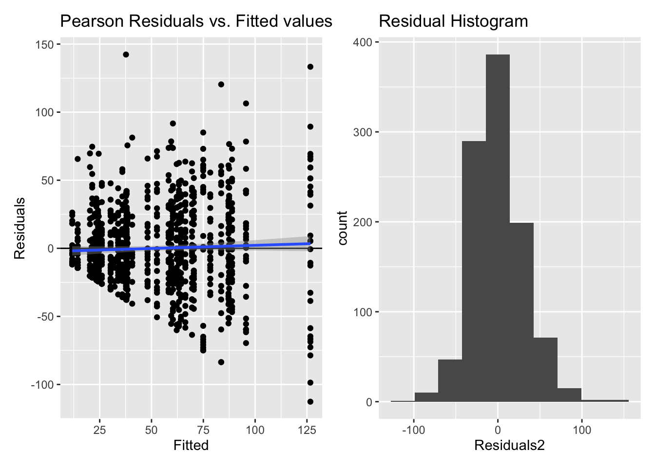
Inf_plots3(x, z %>% drop_na(value), value, transformation = "identity")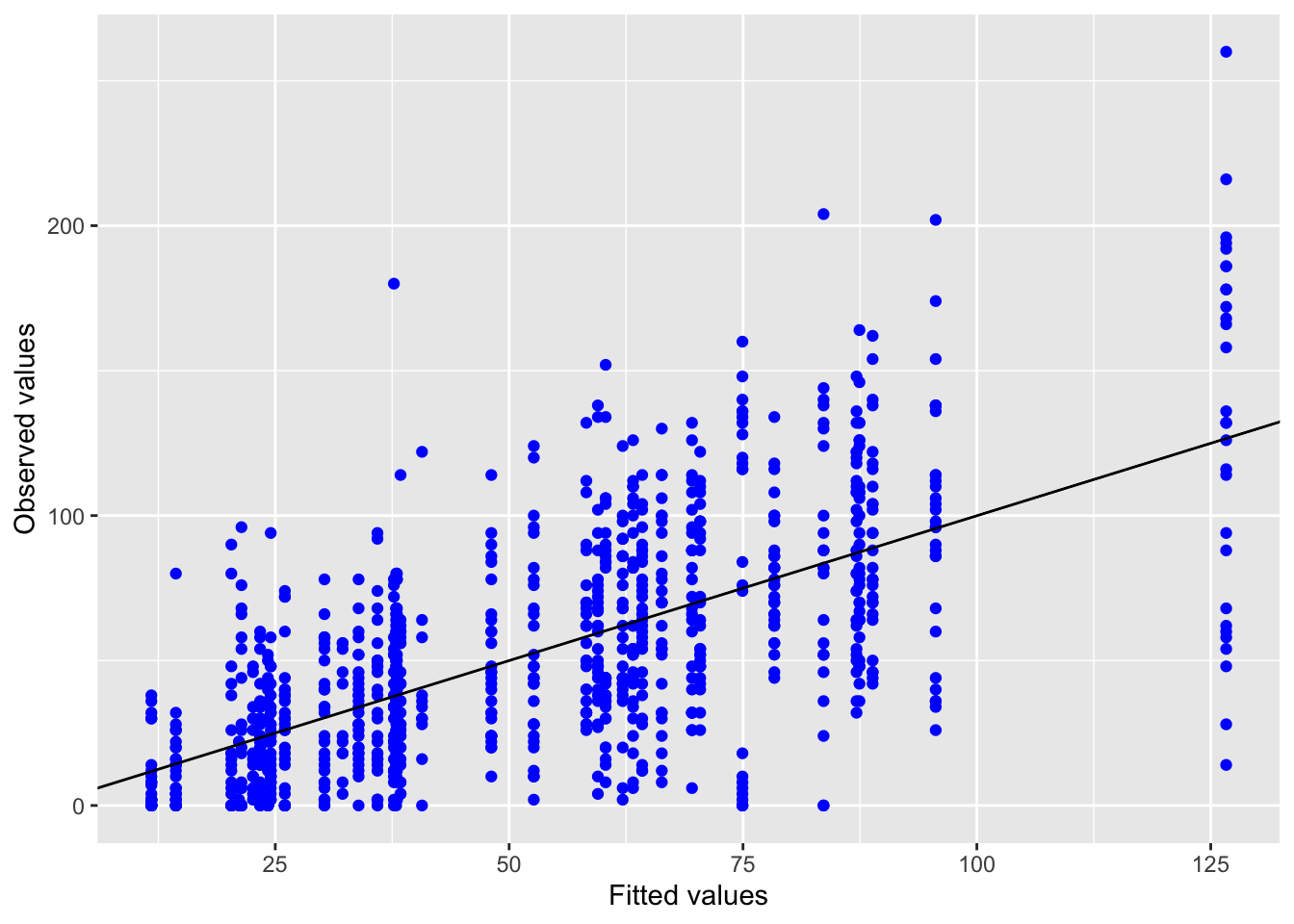
# Inf_plots1(x, z)
Inf_plots2(inference_H2$model[[7]], inference_H2$data[[7]])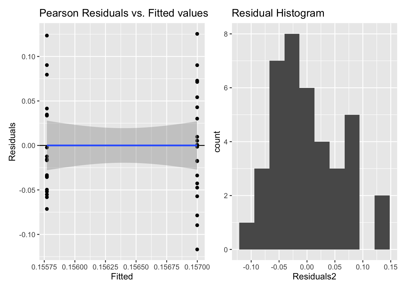
Inf_plots3(inference_H2$model[[7]], inference_H2$data[[7]],
           value, transformation = "identity")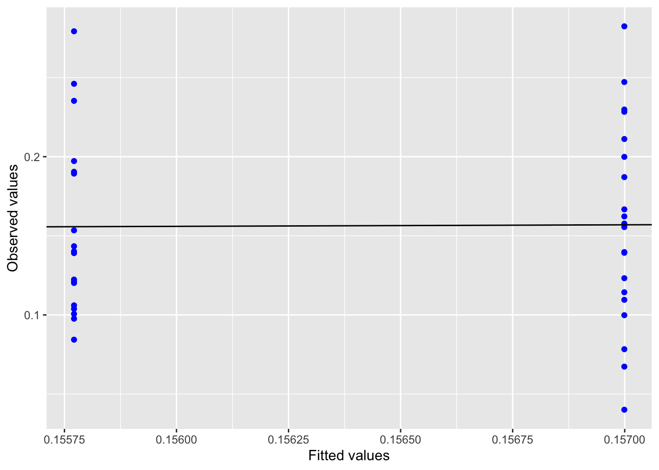
5.2.2.3 Interaction
formula_H2_interaction <- value ~ site*Photoperiod + (1+Photoperiod|site:Id)
formula_H0_interaction <- value ~ site + Photoperiod + (1+Photoperiod|site:Id)

inference_H2.2 <-
  tibble(metric = "log10(daily mean mel EDI)",
         data = metrics %>% filter(metric == "mean") %>% pull(data)) %>%
  mutate(formula_H1 = c(formula_H2_interaction),
         formula_H0 = c(formula_H0_interaction),
         type = "lmer"
         )

inference_H2.2 <-
  inference_H2.2 %>%
  inference_summary2(p_adjustment = 1)

H2_table_interaction <-
Inference_Table(inference_H2.2, p_adjustment = 1, value = value) %>%
  fmt_number(
    c("Intercept", "switzerland", Photoperiodevening, "switzerland:Photoperiodevening"),
    decimals = 2) %>%
  cols_hide(c("cor__Intercept.Photoperiodevening", "sd__Photoperiodevening")) %>%
  cols_align(align = "center", columns = "p.value") %>%
  tab_header(title = "Model Results for Hypothesis 2, Interaction", ) %>%
  tab_footnote(
    "Values were log10 transformed before model fitting"
  ) %>%
  tab_footnote(
    "p-value refers to the interaction effect",
    locations = cells_column_labels(p.value)
  ) %>%
  cols_label(
    Photoperiodevening = "Evening",
    `switzerland:Photoperiodevening` = "Switzerland:Evening") %>%
  cols_add("Day" = 0, .before = Photoperiodevening) %>%
  tab_spanner("Time coeff.", columns = c(Day, Photoperiodevening)) %>%
  tab_spanner("Interaction coeff.", columns = c(`switzerland:Photoperiodevening`)) %>%
  tab_style(
    style = list(
      cell_text(weight = "bold")
    ),
    locations = cells_column_spanners()
  ) %>%
  tab_style(
    style = list(
      cell_text(weight = "bold")
    ),
    locations = cells_column_labels()
  ) %>%
    tab_style(
      style = cell_text(color = pal_jco()(2)[2]),
      locations = cells_column_labels(c("switzerland:Photoperiodevening"))
    )

H2_table_interaction| Model Results for Hypothesis 2, Interaction | ||||||||
|---|---|---|---|---|---|---|---|---|
| p-value1,2 | Intercept |
Site coefficients
|
Time coeff.
|
Interaction coeff.
|
||||
| Malaysia | Switzerland | Day | Evening | Switzerland:Evening | ||||
| log10(daily mean mel EDI) | <0.001 | 2.23 | 0 | 0.41 | 0 | −0.98 | −1.11 |  |
| Values were log10 transformed before model fitting | ||||||||
| 1 p-values are adjusted for multiple comparisons using the false-discovery-rate for n= 1 comparisons | ||||||||
| 2 p-value refers to the interaction effect | ||||||||
v1 <-  gt::extract_cells(H2_table_interaction, 3:8) %>% as.numeric()
v2 <- 10^(v1[1]+v1[3]) %>% round(0)
v3 <- 10^(v1[1]+v1[3] + inference_H2.2$summary[[1]]$estimate[3] +
            inference_H2.2$summary[[1]]$estimate[4])  %>% round(1)
v4 <- 10^(v1[1]) %>% round(0)
v5 <- 10^(v1[1] + inference_H2.2$summary[[1]]$estimate[3]) %>% round(1)
The model reveals that swiss participants have brighter days and darker evenings compared to the malaysia site. Specifically, model prediction is that a swiss participant has a daily mean melanopic EDI during daytime hours of 437 lx, and 3.5 lx during evening hours. An average malaysian participant reaches a mean 170 lx during daytime, and 17.6 lx during evening hours.
5.2.2.3.1 Model diagnostics
Inf_plots1(inference_H2.2$model[[1]], inference_H2.2$data[[1]])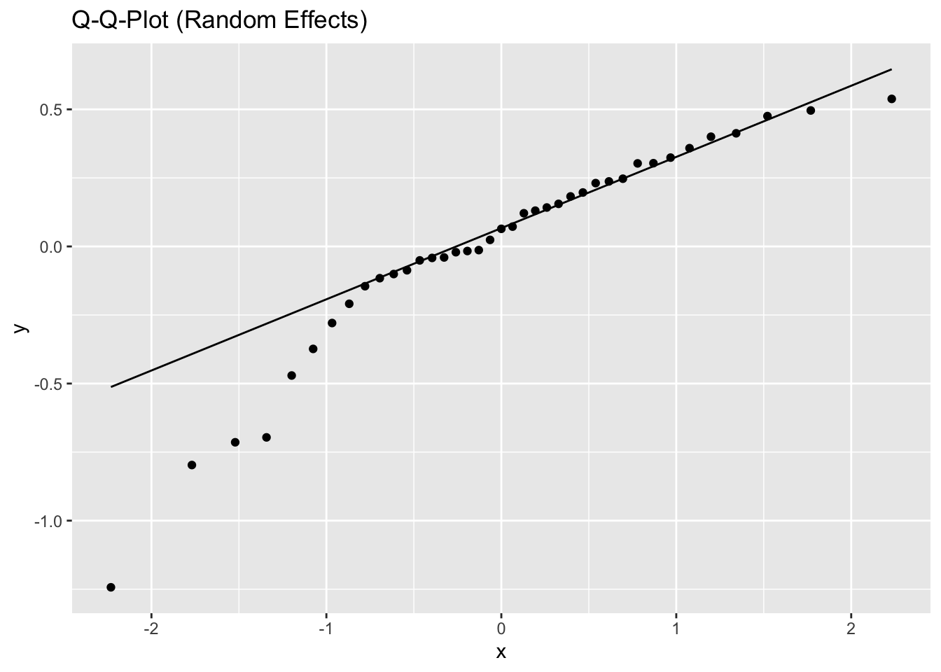
Inf_plots2(inference_H2.2$model[[1]], inference_H2.2$data[[1]])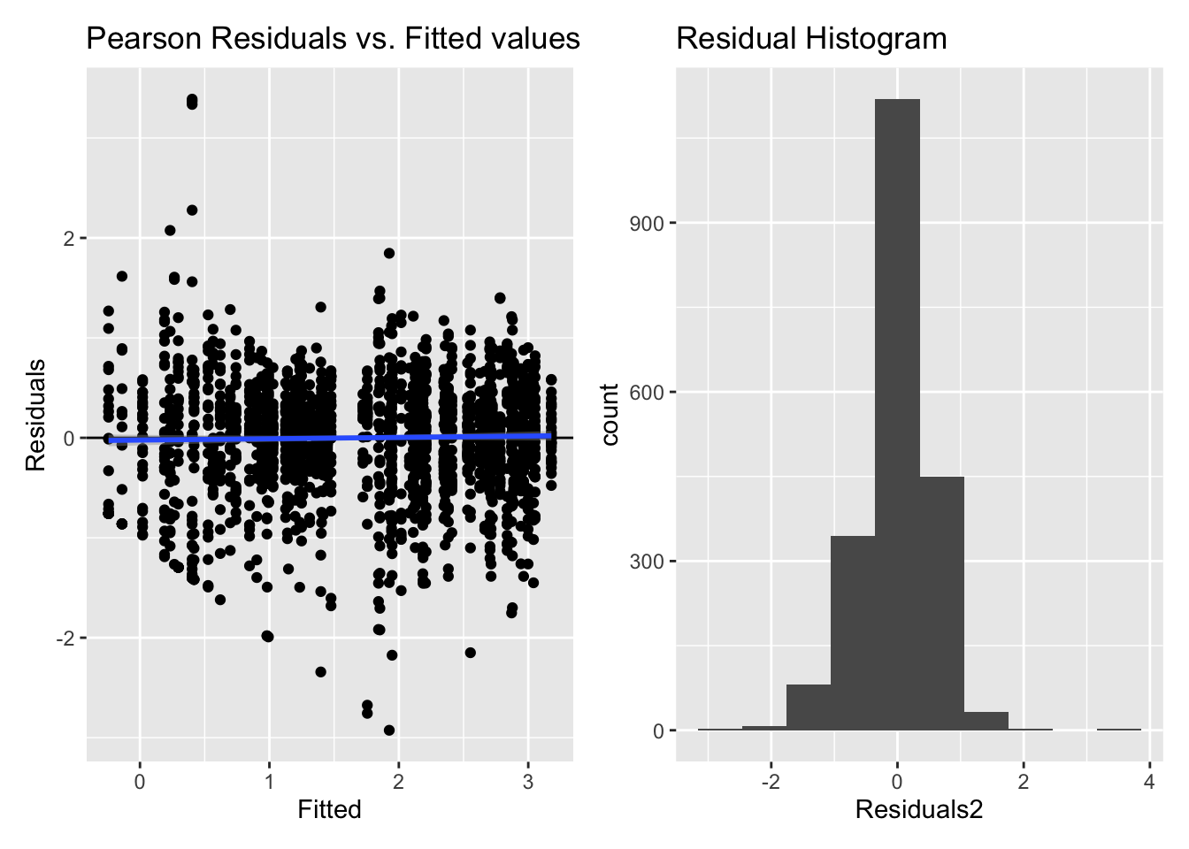
Inf_plots3(inference_H2.2$model[[1]], inference_H2.2$data[[1]] %>%
             drop_na(value), value, transformation = "identity"
           )
5.2.2.4 Pattern
5.2.2.4.1 Metric calculation
metrics <-
  rbind(
    metrics,
    data %>%
      map(\(x) {
        x %>%
          select(Id, Datetime, MEDI) %>%
          mutate(Time = hms::as_hms(Datetime) %>% as.numeric() / 3600,
                 Day = date(Datetime) %>% factor(),
                 Id_day = interaction(Id, Day),
                 metric = "MEDI")
      }) %>%
      list_rbind(names_to = "site") %>%
      mutate(site = factor(site)) %>%
      nest(data = -metric)
  )
5.2.2.4.2 Model fitting
formula_H2_pattern <- log10(MEDI) ~ site + s(Time, by = site, bs = "cc", k=12) + s(Id, by = site, bs = "re")

formula_H0_pattern <- log10(MEDI) ~ s(Time, bs = "cc", k = 12) + s(Id, by = site, bs = "re")

#setting the ends for the cyclic smooth
knots_day <- list(Time = c(0, 24))

#Model generation
Pattern_model0 <-
  bam(formula_H0_pattern,
      data = metrics %>% filter(metric == "MEDI") %>% pull(data) %>% .[[1]],
      knots = knots_day,
      samfrac = 0.1,
      discrete = OpenMP_support,
      nthreads = 4,
      control = list(nthreads = 4))

Pattern_model <-
  bam(formula_H2_pattern,
      data = metrics %>% filter(metric == "MEDI") %>% pull(data) %>% .[[1]],
      knots = knots_day,
      samfrac = 0.1,
      nthreads = 4,
      discrete = OpenMP_support,
      control = list(nthreads = 4))

#Model performance
AICs <-
AIC(Pattern_model, Pattern_model0)
AICs
df AIC
Pattern_model 59.96930 4516274
Pattern_model0 49.97899 4568575Pattern_model_sum <-
summary(Pattern_model)
Pattern_model_sum
Family: gaussian
Link function: identity
Formula:
log10(MEDI) ~ site + s(Time, by = site, bs = "cc", k = 12) +
s(Id, by = site, bs = "re")
Parametric coefficients:
Estimate Std. Error t value Pr(>|t|)
(Intercept) 0.45316 0.05400 8.391 <2e-16 ***
siteswitzerland 0.04480 0.09509 0.471 0.638
---
Signif. codes: 0 '***' 0.001 '**' 0.01 '*' 0.05 '.' 0.1 ' ' 1
Approximate significance of smooth terms:
edf Ref.df F p-value
s(Time):sitemalaysia 9.988 10 37307 <2e-16 ***
s(Time):siteswitzerland 9.993 10 79088 <2e-16 ***
s(Id):sitemalaysia 17.988 18 1623 <2e-16 ***
s(Id):siteswitzerland 18.994 19 2570 <2e-16 ***
---
Signif. codes: 0 '***' 0.001 '**' 0.01 '*' 0.05 '.' 0.1 ' ' 1
R-sq.(adj) = 0.454 Deviance explained = 45.4%
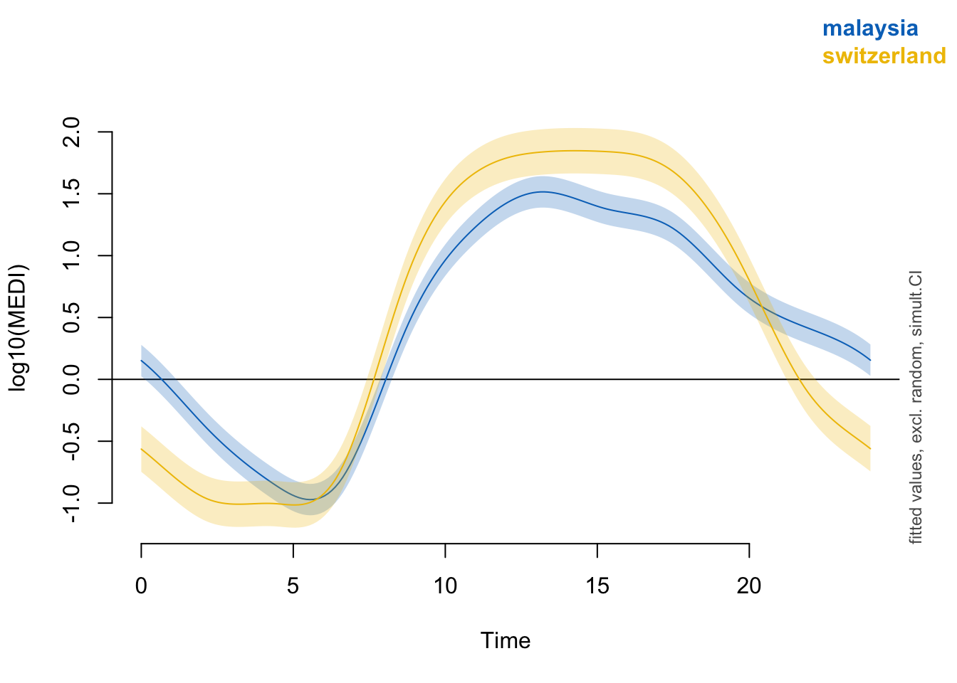
fREML = 2.2583e+06 Scale est. = 1.2648 n = 1469740# plot(Pattern_model)
plot_smooth(
Pattern_model,
view = "Time",
plot_all = "site",
rug = F,
n.grid = 90,
col = pal_jco()(2),
rm.ranef = "s(Id)",
sim.ci = TRUE
)Summary:
* site : factor; set to the value(s): malaysia, switzerland.
* Time : numeric predictor; with 200 values ranging from 0.000000 to 23.983333.
* Id : factor; set to the value(s): MY012.
* NOTE : The following random effects columns are canceled: s(Time):sitemalaysia,s(Time):siteswitzerland,s(Id):sitemalaysia,s(Id):siteswitzerland
* Simultaneous 95%-CI used :
Critical value: 2.343
Proportion posterior simulations in pointwise CI: 0.87 (10000 samples)
Proportion posterior simulations in simultaneous CI: 0.95 (10000 samples)
plot_diff(Pattern_model,
          view = "Time",
          rm.ranef = "s(Id)",
          comp = list(site = c("malaysia", "switzerland")),
          sim.ci = TRUE)
Summary:
* Time : numeric predictor; with 200 values ranging from 0.000000 to 23.983333.
* Id : factor; set to the value(s): MY012.
* NOTE : The following random effects columns are canceled: s(Time):sitemalaysia,s(Time):siteswitzerland,s(Id):sitemalaysia,s(Id):siteswitzerland
* Simultaneous 95%-CI used :
Critical value: 2.099
Proportion posterior simulations in pointwise CI: 1 (10000 samples)
Proportion posterior simulations in simultaneous CI: 1 (10000 samples)
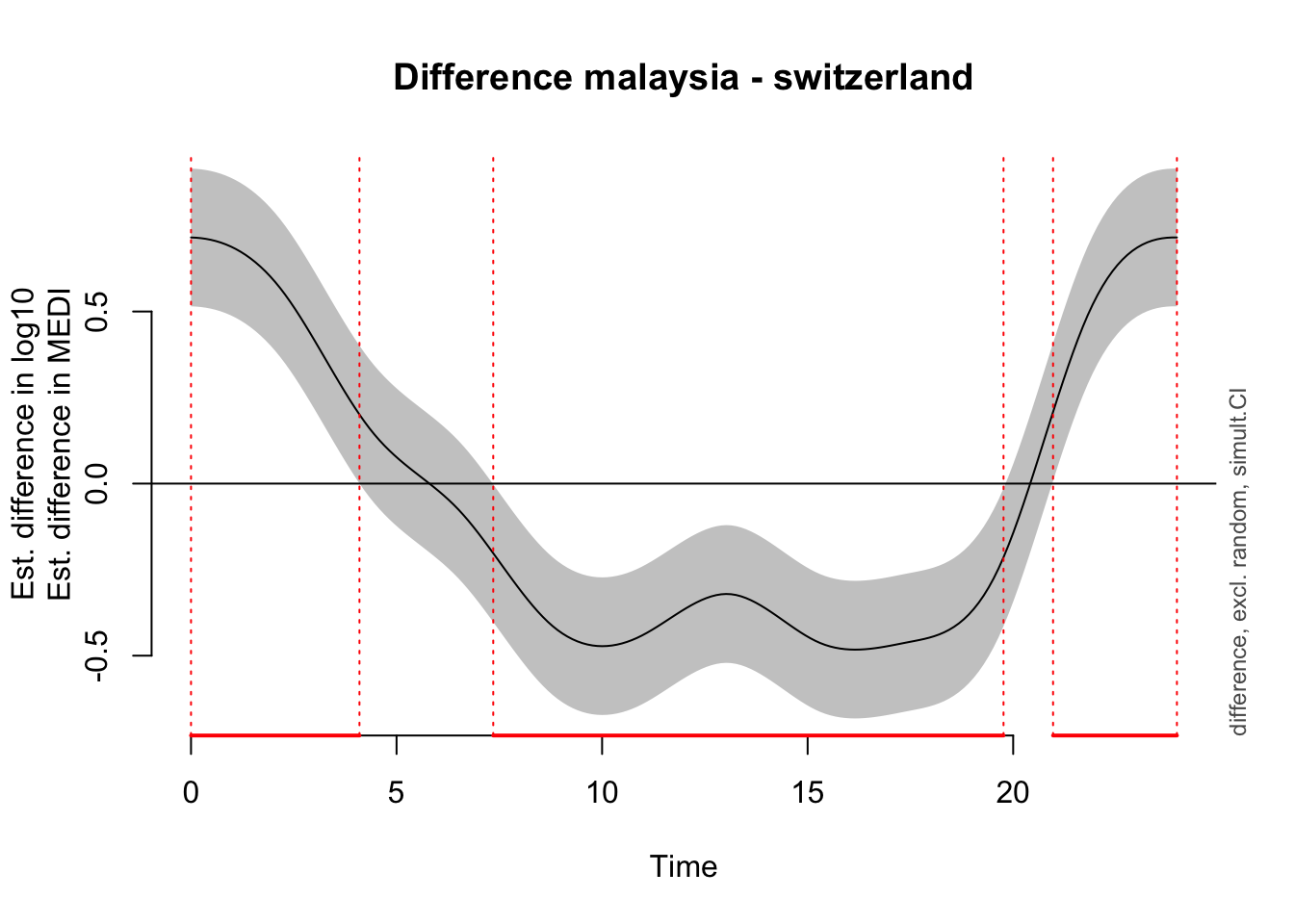
Time window(s) of significant difference(s):
    0.000000 - 4.097655
    7.351675 - 19.765159
    20.970352 - 23.983333
5.2.2.5 Model Diagnostics
gam.check(Pattern_model, rep = 100)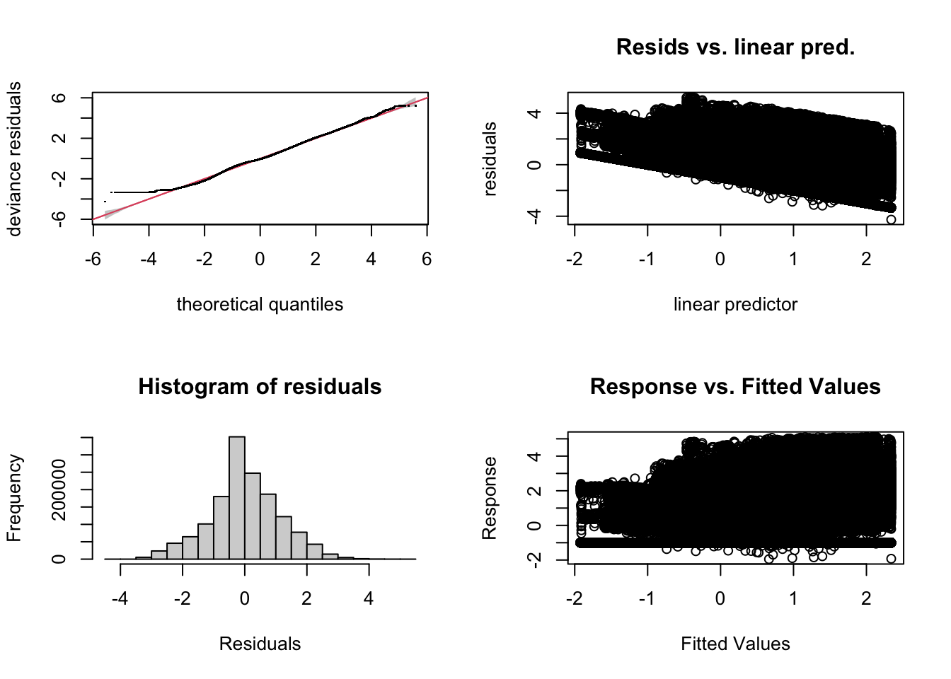
Method: fREML   Optimizer: perf chol
$grad
[1]  2.384107e-06  4.512179e-05  9.560424e-10  3.769323e-07 -4.802411e-05

$hess
           [,1]          [,2]          [,3]          [,4]          [,5]
   4.986919e+00 -3.355115e-25  2.662657e-06 -3.765739e-22     -4.994000
   3.004535e-26  4.991019e+00 -5.625615e-23  4.495121e-07     -4.996344
   2.662657e-06  6.353030e-23  8.987577e+00  7.130559e-20     -8.993804
  -1.189254e-22  4.495121e-07  9.619634e-21  9.488433e+00     -9.497046
d -4.994000e+00 -4.996344e+00 -8.993804e+00 -9.497046e+00 734869.000048

Model rank =  100 / 100

Basis dimension (k) checking results. Low p-value (k-index<1) may
indicate that k is too low, especially if edf is close to k'.

                           k'   edf k-index p-value
s(Time):sitemalaysia    10.00  9.99    1.01    0.70
s(Time):siteswitzerland 10.00  9.99    1.01    0.67
s(Id):sitemalaysia      39.00 17.99      NA      NA
s(Id):siteswitzerland   39.00 18.99      NA      NA
formula_H2_pattern <- log10(MEDI) ~
site + s(Time, by = site, bs = "cc", k=12) +
s(Time, by = Id, bs = "cc", k = 12) +
s(Id, by = site, bs = "re")
formula_H0_pattern <- log10(MEDI) ~
s(Time, bs = "cc", k = 12) +
s(Time, by = Id, bs = "cc", k = 12) +
s(Id, by = site, bs = "re")
formula_Hm1_pattern <- log10(MEDI) ~
s(Time, by = Id, bs = "cc", k = 12) +
s(Id, by = site, bs = "re")
#setting the ends for the cyclic smooth
knots_day <- list(Time = c(0, 24))
#Model generation
Pattern_model0 <-
bam(formula_H0_pattern,
data = metrics %>% filter(metric == "MEDI") %>% pull(data) %>% .[[1]],
knots = knots_day,
samfrac = 0.1,
discrete = OpenMP_support,
nthreads = 4,
control = list(nthreads = 4))
Pattern_modelm1 <-
bam(formula_Hm1_pattern,
data = metrics %>% filter(metric == "MEDI") %>% pull(data) %>% .[[1]],
knots = knots_day,
samfrac = 0.1,
discrete = OpenMP_support,
nthreads = 4,
control = list(nthreads = 4))
Pattern_modelm2 <-
bam(formula_H2_pattern,
data = metrics %>% filter(metric == "MEDI") %>% pull(data) %>% .[[1]],
knots = knots_day,
samfrac = 0.1,
nthreads = 4,
discrete = OpenMP_support,
control = list(nthreads = 4))
#Model performance
AICs <-
AIC(Pattern_modelm2, Pattern_model0, Pattern_modelm1)
AICs df AIC
Pattern_modelm2 427.2126 4334753
Pattern_model0 427.3398 4334745
Pattern_modelm1 428.0966 4334743Pattern_model_sum <-
summary(Pattern_modelm2)
Pattern_model_sum
Family: gaussian
Link function: identity

Formula:
log10(MEDI) ~ site + s(Time, by = site, bs = "cc", k = 12) +
    s(Time, by = Id, bs = "cc", k = 12) + s(Id, by = site, bs = "re")

Parametric coefficients:
                Estimate Std. Error t value Pr(>|t|)
(Intercept)      0.45343    0.05409   8.383   <2e-16 ***
siteswitzerland  0.04433    0.09500   0.467    0.641
---
Signif. codes:  0 '***' 0.001 '**' 0.01 '*' 0.05 '.' 0.1 ' ' 1

Approximate significance of smooth terms:
                              edf Ref.df        F p-value
s(Time):sitemalaysia    9.154e+00     10   10.872  <2e-16 ***
s(Time):siteswitzerland 9.966e+00     10 5989.456  <2e-16 ***
s(Time):IdMY001         9.669e+00     10   26.664  <2e-16 ***
s(Time):IdMY002         9.790e+00     10   31.793  <2e-16 ***
s(Time):IdMY003         7.647e+00     10    3.150  <2e-16 ***
s(Time):IdMY004         9.581e+00     10   22.191  <2e-16 ***
s(Time):IdMY005         9.432e+00     10   14.535  <2e-16 ***
s(Time):IdMY007         9.632e+00     10   25.656  <2e-16 ***
s(Time):IdMY008         9.765e+00     10   32.729  <2e-16 ***
s(Time):IdMY009         8.340e+00     10    4.870  <2e-16 ***
s(Time):IdMY010         9.825e+00     10   41.545  <2e-16 ***
s(Time):IdMY011         9.688e+00     10   29.210  <2e-16 ***
s(Time):IdMY012         9.680e+00     10   27.202  <2e-16 ***
s(Time):IdMY013         8.956e+00     10    8.589  <2e-16 ***
s(Time):IdMY014         9.014e+00     10    9.024  <2e-16 ***
s(Time):IdMY015         9.737e+00     10   30.400  <2e-16 ***
s(Time):IdMY016         9.587e+00     10   22.074  <2e-16 ***
s(Time):IdMY017         9.579e+00     10   18.883  <2e-16 ***
s(Time):IdMY018         9.680e+00     10   20.209  <2e-16 ***
s(Time):IdMY019         9.828e+00     10   46.858  <2e-16 ***
s(Time):IdMY020         9.270e+00     10    9.067  <2e-16 ***
s(Time):IdID01          9.885e+00     10  271.241  <2e-16 ***
s(Time):IdID02          9.887e+00     10   92.928  <2e-16 ***
s(Time):IdID03          9.974e+00     10  430.152  <2e-16 ***
s(Time):IdID04          9.976e+00     10 1263.553  <2e-16 ***
s(Time):IdID05          9.939e+00     10  195.099  <2e-16 ***
s(Time):IdID06          9.748e+00     10  144.720  <2e-16 ***
s(Time):IdID07          9.908e+00     10  145.609  <2e-16 ***
s(Time):IdID08          9.909e+00     10  230.906  <2e-16 ***
s(Time):IdID09          9.683e+00     10 1242.976  <2e-16 ***
s(Time):IdID10          9.801e+00     10  332.364  <2e-16 ***
s(Time):IdID11          9.955e+00     10  265.852  <2e-16 ***
s(Time):IdID12          9.873e+00     10   95.177  <2e-16 ***
s(Time):IdID13          9.965e+00     10  334.103  <2e-16 ***
s(Time):IdID14          9.919e+00     10  434.586  <2e-16 ***
s(Time):IdID15          9.853e+00     10  397.519  <2e-16 ***
s(Time):IdID16          1.555e-04     10    0.000  <2e-16 ***
s(Time):IdID17          9.935e+00     10  635.199  <2e-16 ***
s(Time):IdID18          9.819e+00     10  239.344  <2e-16 ***
s(Time):IdID19          9.897e+00     10  265.421  <2e-16 ***
s(Time):IdID20          9.954e+00     10  789.975  <2e-16 ***
s(Id):sitemalaysia      1.799e+01     18 1837.369  <2e-16 ***
s(Id):siteswitzerland   1.899e+01     19 2895.488  <2e-16 ***
---
Signif. codes:  0 '***' 0.001 '**' 0.01 '*' 0.05 '.' 0.1 ' ' 1

R-sq.(adj) =  0.518   Deviance explained = 51.8%
fREML = 2.1686e+06  Scale est. = 1.1176    n = 1469740
#Model overview
# plot(Pattern_model, shade = TRUE, residuals = TRUE, cex = 1, all.terms = TRUE)
colors_pattern <- pal_jco()(2)
plot_smooth(
Pattern_modelm1,
view = "Time",
plot_all = "Id",
rm.ranef = FALSE,
se = 0,
rug = F,
n.grid = 90,
col = c(rep(colors_pattern[1], 19),rep(colors_pattern[2], 20)),
# sim.ci = TRUE
)Summary:
* Time : numeric predictor; with 90 values ranging from 0.000000 to 23.983333.
* Id : factor with 39 values; set to the value(s): ID01, ID02, ID03, ID04, ID05, ID06, ID07, ID08, ID09, ID10, ...
* site : factor; set to the value(s): switzerland. 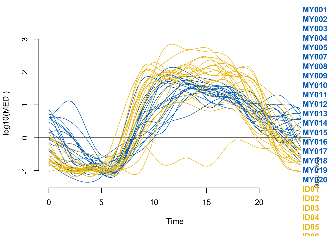
5.2.2.6 Model Diagnostics
gam.check(Pattern_model)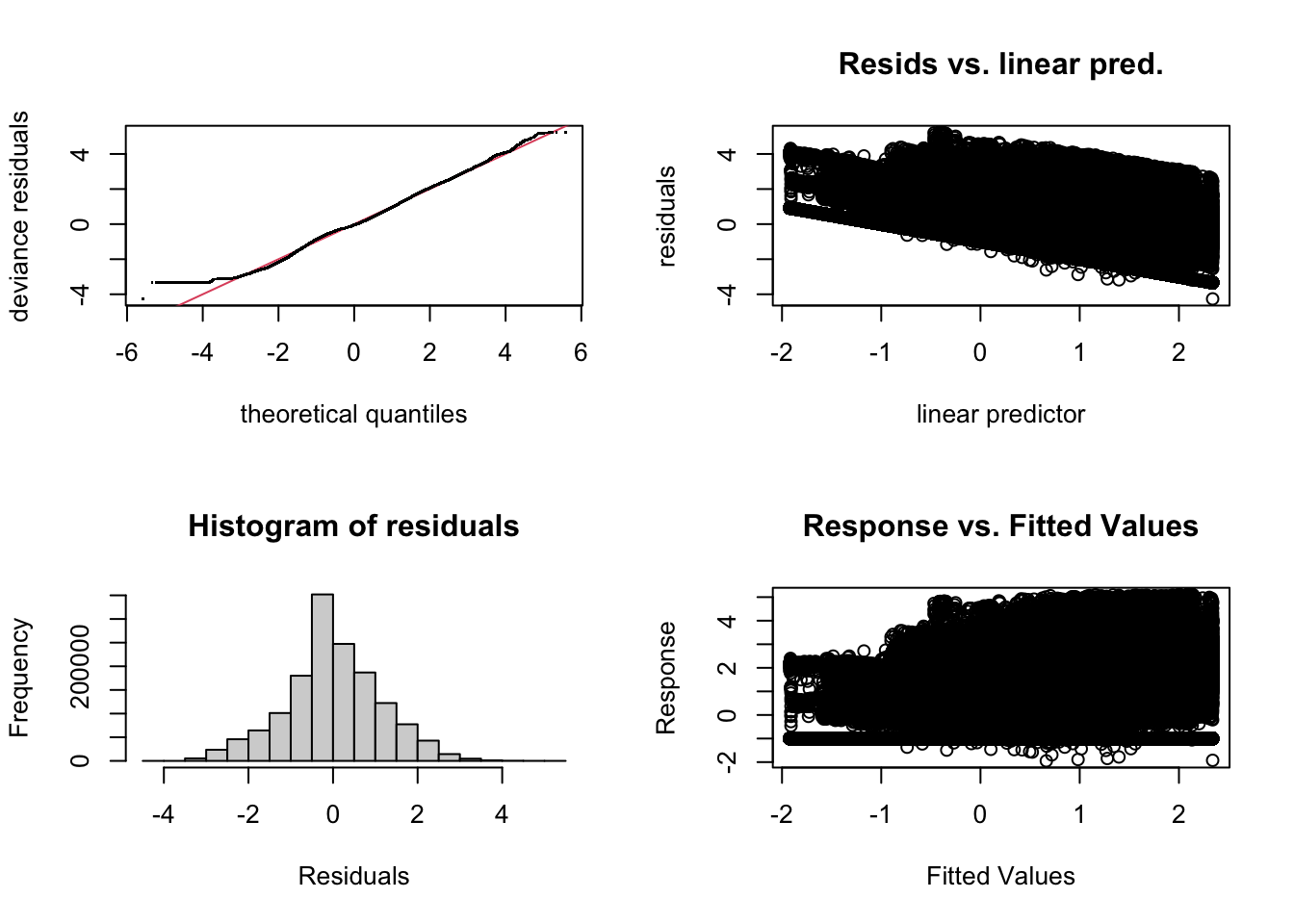
Method: fREML   Optimizer: perf chol
$grad
[1]  2.384107e-06  4.512179e-05  9.560424e-10  3.769323e-07 -4.802411e-05

$hess
           [,1]          [,2]          [,3]          [,4]          [,5]
   4.986919e+00 -3.355115e-25  2.662657e-06 -3.765739e-22     -4.994000
   3.004535e-26  4.991019e+00 -5.625615e-23  4.495121e-07     -4.996344
   2.662657e-06  6.353030e-23  8.987577e+00  7.130559e-20     -8.993804
  -1.189254e-22  4.495121e-07  9.619634e-21  9.488433e+00     -9.497046
d -4.994000e+00 -4.996344e+00 -8.993804e+00 -9.497046e+00 734869.000048

Model rank =  100 / 100

Basis dimension (k) checking results. Low p-value (k-index<1) may
indicate that k is too low, especially if edf is close to k'.

                           k'   edf k-index p-value
s(Time):sitemalaysia    10.00  9.99    1.01    0.76
s(Time):siteswitzerland 10.00  9.99    1.01    0.76
s(Id):sitemalaysia      39.00 17.99      NA      NA
s(Id):siteswitzerland   39.00 18.99      NA      NA
Using the formula specified in the preregistration document reveals no significant difference between the sites (∆AIC < 2 for the more complex model). Furthermore, a reduced model only including individual smooths per participant (Pattern_modelm1) reveals no common pattern over time, i.e. the patterns vary so strongly between participants, that the model suffers when trying to extract common values at a given time point.
To nonetheless illustrate the overall trend between the sites, a simplified model is used, that only implements random intercepts for the participants (compared to random smooths in the preregistration variant). This allows for an overall comparison between the sites, even though it can not be mapped 1:1 on individual participants. Here, there is strong evidence for the effect of site, and the difference is significant across most of the day. The difference-plot shows that malaysian participants show lower MEDI values during the day compared to swiss participants, and higher ones at night.
5.3 Research Question 2
RQ 2: Are there differences in self-reported light exposure patterns using LEBA across time or between the two sites, and if so, in which questions/scores?
As RQ relates to LEBA questions and factors, factors have to be calculated first.
5.3.0.1 Metric calculation
p_adjustment <- append(
  p_adjustment,
  list(
  H3 = 23+5
))


#Factor calculation
factors_leba <- list(
  F1 = names(leba_questions)[c(1,2,3)],
  F2 = names(leba_questions)[c(4:9)],
  F3 = names(leba_questions)[c(10:14)],
  F4 = names(leba_questions)[c(15:18)],
  F5 = names(leba_questions)[c(19:23)]
)
Fs <- paste0("F", 1:5)

leba_data_combined <-
leba_data_combined %>%
  mutate(leba_F2_04 = fct_rev(leba_F2_04),
         leba_F1 = rowSums(across(contains(factors_leba$F1), as.numeric)),
         leba_F2 = rowSums(across(contains(factors_leba$F2), as.numeric)),
         leba_F3 = rowSums(across(contains(factors_leba$F3), as.numeric)),
         leba_F4 = rowSums(across(contains(factors_leba$F4), as.numeric)),
         leba_F5 = rowSums(across(contains(factors_leba$F5), as.numeric)),
         ) %>%
  mutate(leba_F2_04 = fct_rev(leba_F2_04),
         across(c(site, Id), factor))

leba_factors <- c(
  leba_F1 = "Wearing blue light filtering glasses indoors and outdoors",
  leba_F2 = "Spending time outdoors",
  leba_F3 = "Using phones and smartwatches in bed before sleep",
  leba_F4 = "Controlling and using ambient light before bedtime",
  leba_F5 = "Using light in the morning and during daytime"
)

#set variable labels
var_label(leba_data_combined) <- leba_factors %>% as.list()

leba_metrics <-
  leba_data_combined %>%
  mutate(across(contains("leba_F"), as.numeric)) %>%
  pivot_longer(cols = starts_with("leba_F"), names_to = "metric", values_to = "value") %>%
  nest(data = -metric)

leba_metrics <-
leba_metrics %>%
  rowwise() %>%
  mutate(data = list({
    if(str_length(metric) == 7) data
    else data %>% mutate(value = factor(value, levels = 1:5, labels = leba_levels))
  }
  ))
5.3.1 Hypothesis 3
\(H3\): There are differences in LEBA items and factors between Malaysia and Switzerland.
5.3.1.1 Model fitting
5.3.1.1.1 Whole Dataset
formula_H3 <- value ~ site + (1|site:Id)
formula_H0 <- value ~ 1 + (1|site:Id)

clmm <- ordinal::clmm

inference_H3 <-
leba_metrics %>%
  filter(str_length(metric) != 7) %>%
  mutate(formula_H1 = c(formula_H3),
         formula_H0 = c(formula_H0),
         type = "clmm")

inference_H3 <-
  inference_H3 %>%
    rowwise() %>%
    mutate(
      model =
        list(
            do.call(type, list(formula = formula_H1,
                                          data = data,
                               nAGQ = 5))
            ),
      model0 = list(
        do.call(type, list(formula = formula_H0,
                           data = data,
                           nAGQ = 5))
      ))

inference_H3$comparison <- vector("list", nrow(inference_H3))

for(i in 1:nrow(inference_H3)) {
  comparison <- anova(inference_H3$model[[i]], inference_H3$model0[[i]])
  inference_H3$comparison[[i]] <- comparison
}

inference_H3 <-
inference_H3 %>%
  mutate(
      p.value_adj = comparison$`Pr(>Chisq)` %>% .[2] %>%
        p.adjust(method = "fdr", n = p_adjustment$H3),
      significant = p.value_adj <= 0.05,
      summary = list(
        switch(significant+1,
               tidy(model0),
               tidy(model))),
    table = list(
        tibble(
          metric = metric,
          p.value =
            p.value_adj %>%
            style_pvalue() %>%
            {ifelse(significant, paste0("**", ., "**"),.)},
          summary %>%
            mutate(estimate = estimate) %>%
            select(term, estimate) %>%
            filter(term != "sd__(Intercept)" &
                     term != "sd__Observation") %>%
            mutate(term = str_remove_all(term, "\\(|\\)|site")) %>%
            pivot_wider(names_from = term, values_from = estimate)
        ) %>%
          mutate(malaysia = if(exists("switzerland")) 0 else NA)
  )
  )

inference_H3 %>% pull(table) %>% list_rbind() %>% select(metric, p.value) %>% gt()| metric | p.value |
|---|---|
| leba_F1_01 | >0.9 |
| leba_F1_02 | >0.9 |
| leba_F1_03 | >0.9 |
| leba_F2_04 | >0.9 |
| leba_F2_05 | >0.9 |
| leba_F2_06 | >0.9 |
| leba_F2_07 | >0.9 |
| leba_F2_08 | >0.9 |
| leba_F2_09 | 0.8 |
| leba_F3_10 | >0.9 |
| leba_F3_11 | >0.9 |
| leba_F3_12 | 0.7 |
| leba_F3_13 | >0.9 |
| leba_F3_14 | >0.9 |
| leba_F4_15 | >0.9 |
| leba_F4_16 | >0.9 |
| leba_F4_17 | 0.5 |
| leba_F4_18 | >0.9 |
| leba_F5_19 | >0.9 |
| leba_F5_20 | 0.9 |
| leba_F5_21 | >0.9 |
| leba_F5_22 | 0.3 |
| leba_F5_23 | >0.9 |
Under the strict p-value adjustment for H3 (n=28), none of the behavioral questions are significantly different.
5.3.1.1.2 Only last collection point
formula_H3 <- value ~ site
formula_H0 <- value ~ 1

clmm <- ordinal::clmm
clm <- ordinal::clm

inference_H3.2 <-
leba_metrics %>%
  filter(str_length(metric) != 7) %>%
  mutate(formula_H1 = c(formula_H3),
         formula_H0 = c(formula_H0),
         type = "clm",
         data = list(data %>% filter(Day == 31)))

inference_H3.2 <-
  inference_H3.2 %>%
    rowwise() %>%
    mutate(
      model =
        list(
            do.call(type, list(formula = formula_H1,
                                          data = data))
            ),
      model0 = list(
        do.call(type, list(formula = formula_H0,
                           data = data))
      ))

inference_H3.2$comparison <- vector("list", nrow(inference_H3.2))

for(i in 1:nrow(inference_H3.2)) {
  comparison <- anova(inference_H3.2$model[[i]], inference_H3.2$model0[[i]])
  inference_H3.2$comparison[[i]] <- comparison
}

inference_H3.2 <-
inference_H3.2 %>%
  mutate(
      p.value_adj = comparison$`Pr(>Chisq)` %>% .[2] %>%
        p.adjust(method = "fdr", n = p_adjustment$H3),
      significant = p.value_adj <= 0.05,
      summary = list(
        switch(significant+1,
               tidy(model0),
               tidy(model))),
    table = list(
        tibble(
          metric = metric,
          p.value =
            p.value_adj %>%
            style_pvalue() %>%
            {ifelse(significant, paste0("**", ., "**"),.)},
          summary %>%
            mutate(estimate = estimate) %>%
            select(term, estimate) %>%
            filter(term != "sd__(Intercept)" &
                     term != "sd__Observation") %>%
            mutate(term = str_remove_all(term, "\\(|\\)|site")) %>%
            pivot_wider(names_from = term, values_from = estimate)
        ) %>%
          mutate(malaysia = if(exists("switzerland")) 0 else NA)
  )
  )

inference_H3.2 %>% pull(table) %>% list_rbind() %>% select(metric, p.value) %>% gt()| metric | p.value |
|---|---|
| leba_F1_01 | >0.9 |
| leba_F1_02 | >0.9 |
| leba_F1_03 | >0.9 |
| leba_F2_04 | >0.9 |
| leba_F2_05 | >0.9 |
| leba_F2_06 | >0.9 |
| leba_F2_07 | >0.9 |
| leba_F2_08 | >0.9 |
| leba_F2_09 | >0.9 |
| leba_F3_10 | >0.9 |
| leba_F3_11 | >0.9 |
| leba_F3_12 | 0.055 |
| leba_F3_13 | >0.9 |
| leba_F3_14 | >0.9 |
| leba_F4_15 | >0.9 |
| leba_F4_16 | >0.9 |
| leba_F4_17 | >0.9 |
| leba_F4_18 | >0.9 |
| leba_F5_19 | >0.9 |
| leba_F5_20 | >0.9 |
| leba_F5_21 | >0.9 |
| leba_F5_22 | >0.9 |
| leba_F5_23 | >0.9 |
formula_H3 <- value ~ site + (1|site:Id)
formula_H0 <- value ~ 1 + (1|site:Id)

inference_H3.3 <-
  leba_metrics %>%
  filter(str_length(metric) == 7) %>%
  mutate(formula_H1 = c(formula_H3),
         formula_H0 = c(formula_H0),
         type = "lmer",
         family = list(poisson())
         )

inference_H3.3 <-
  inference_H3.3 %>%
  inference_summary2(p_adjustment = p_adjustment$H3)

inference_H3.3 %>% pull(table) %>% list_rbind() %>% select(metric, p.value) %>% gt()| metric | p.value |
|---|---|
| leba_F1 | >0.9 |
| leba_F2 | >0.9 |
| leba_F3 | >0.9 |
| leba_F4 | >0.9 |
| leba_F5 | >0.9 |
Under the strict p-value adjustment for H3 (n=28), none of the behavioral factors are significantly different between sites.
5.3.1.1.3 Model diagnostics
Inf_plots1(x, z)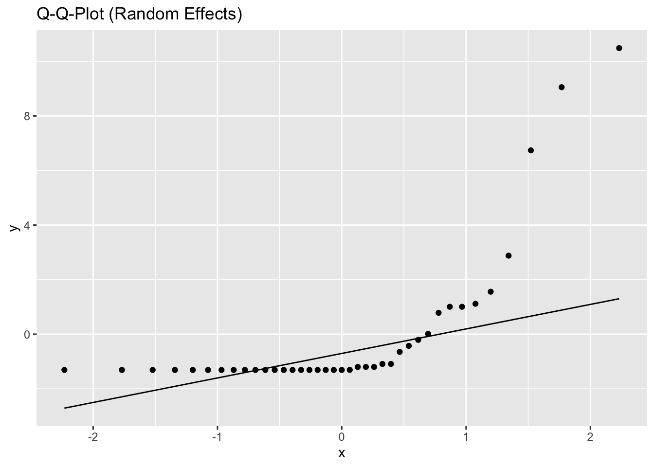
Inf_plots2(x, z)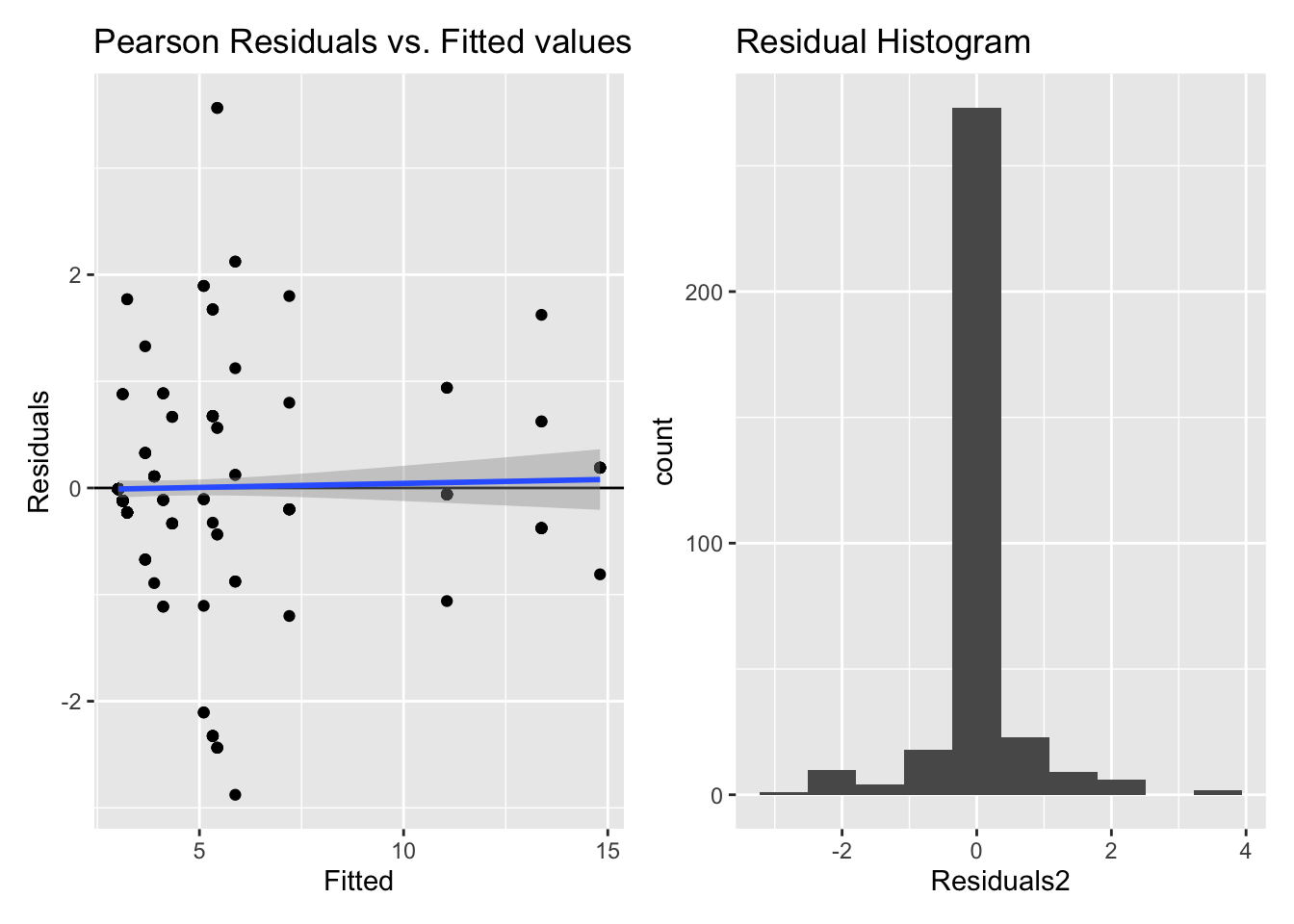
Inf_plots3(x, z, value, "identity")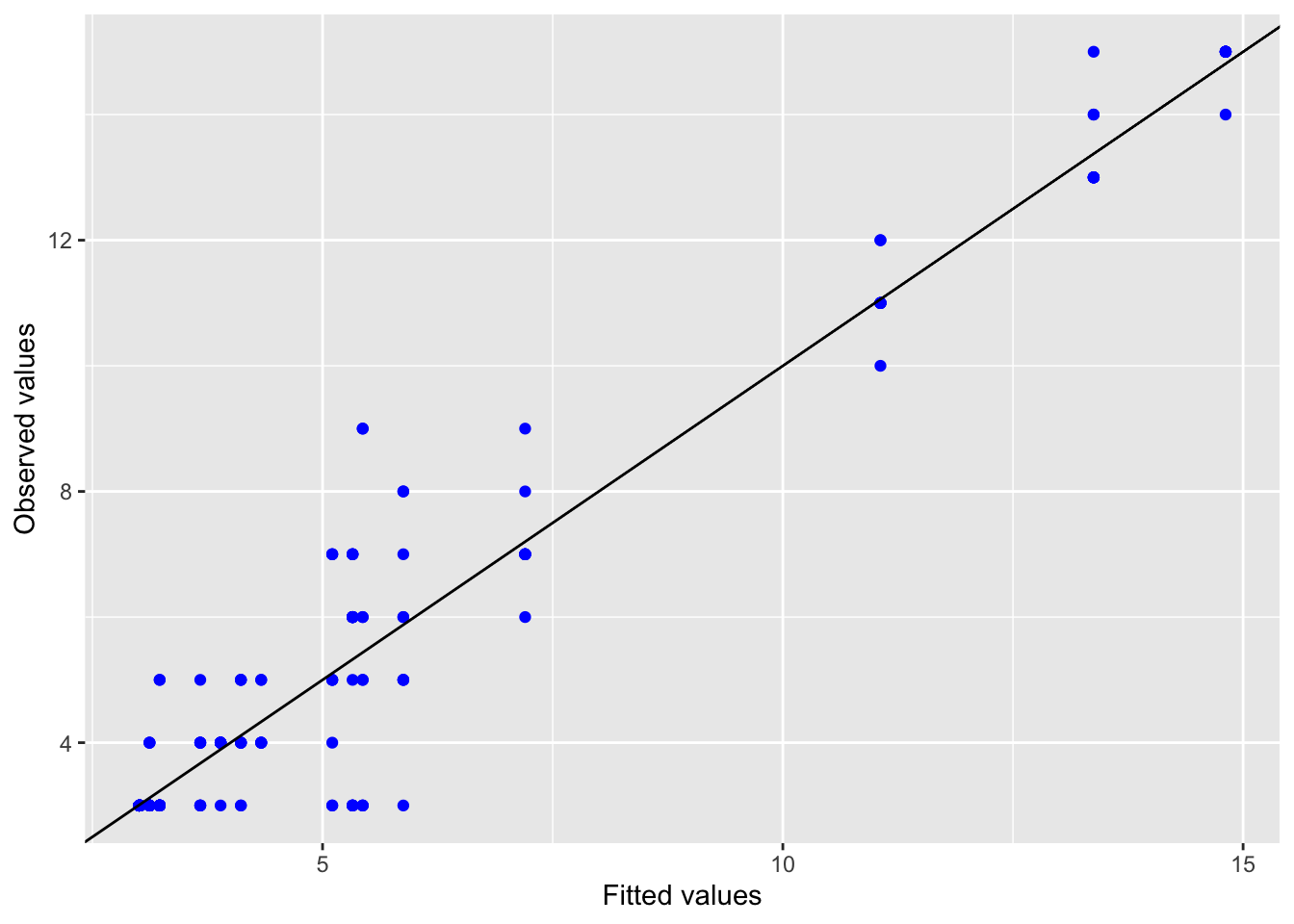
Inf_plots1(x, z)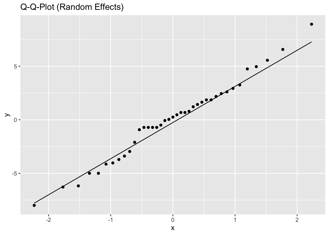
Inf_plots2(x, z)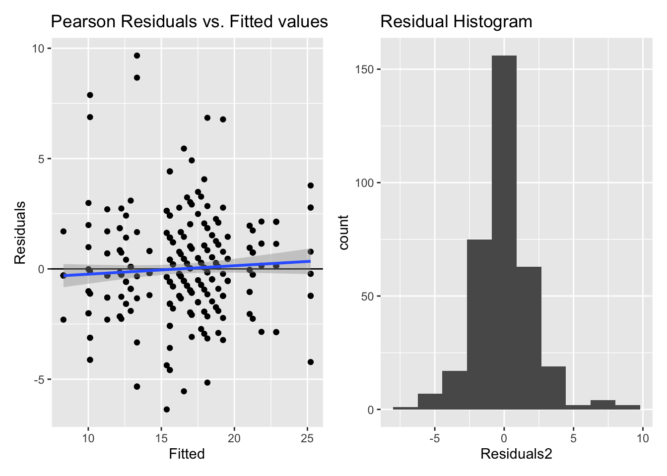
Inf_plots3(x, z, value, "identity")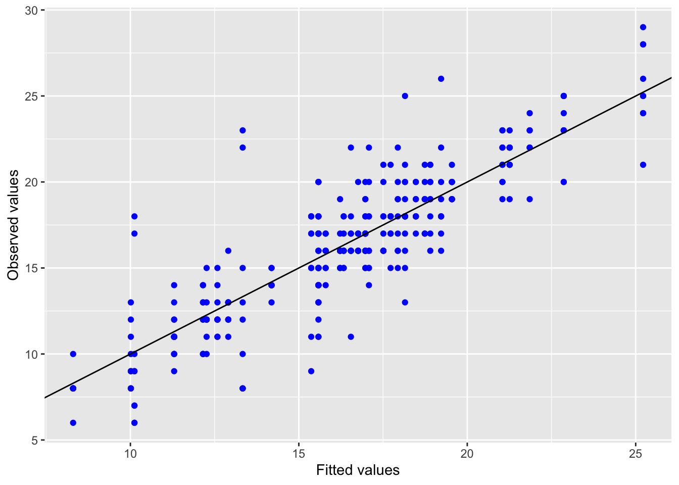
Inf_plots1(x, z)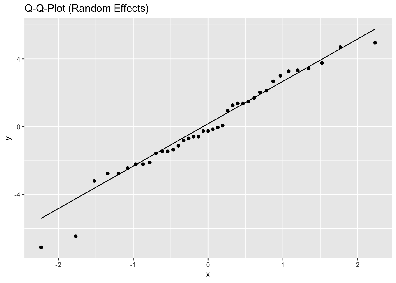
Inf_plots2(x, z)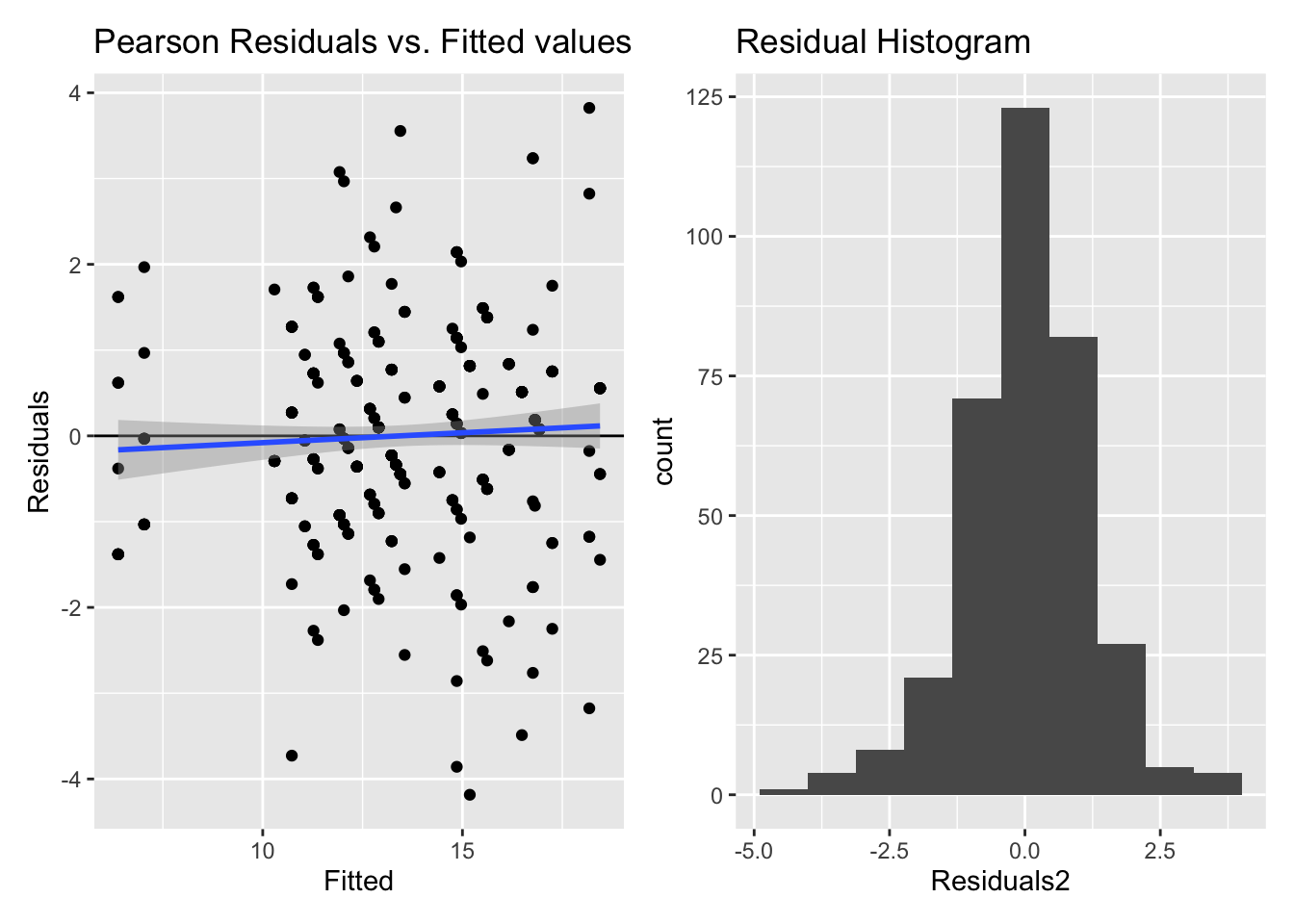
Inf_plots3(x, z, value, "identity")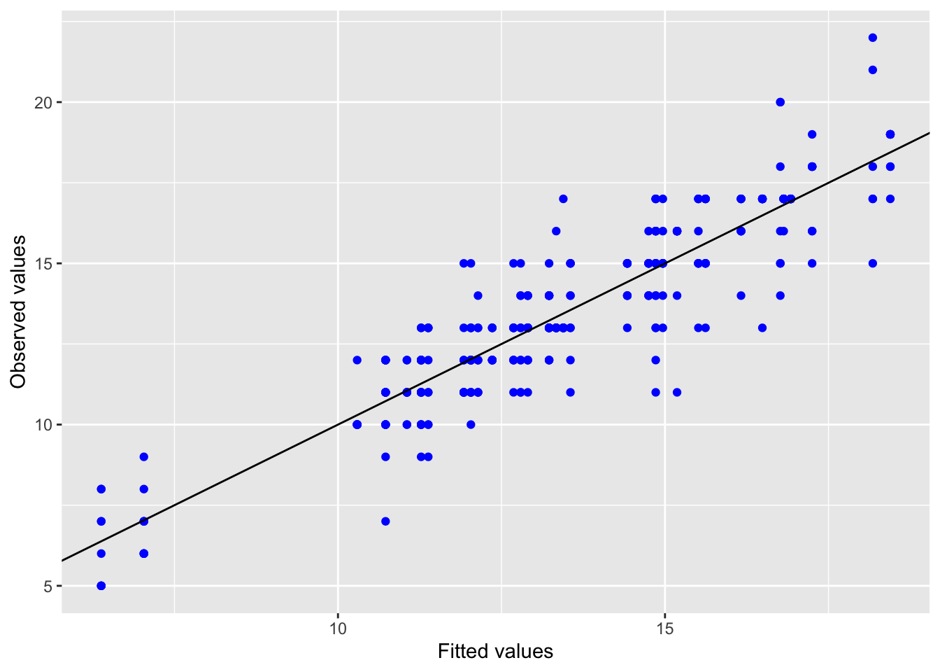
Inf_plots1(x, z)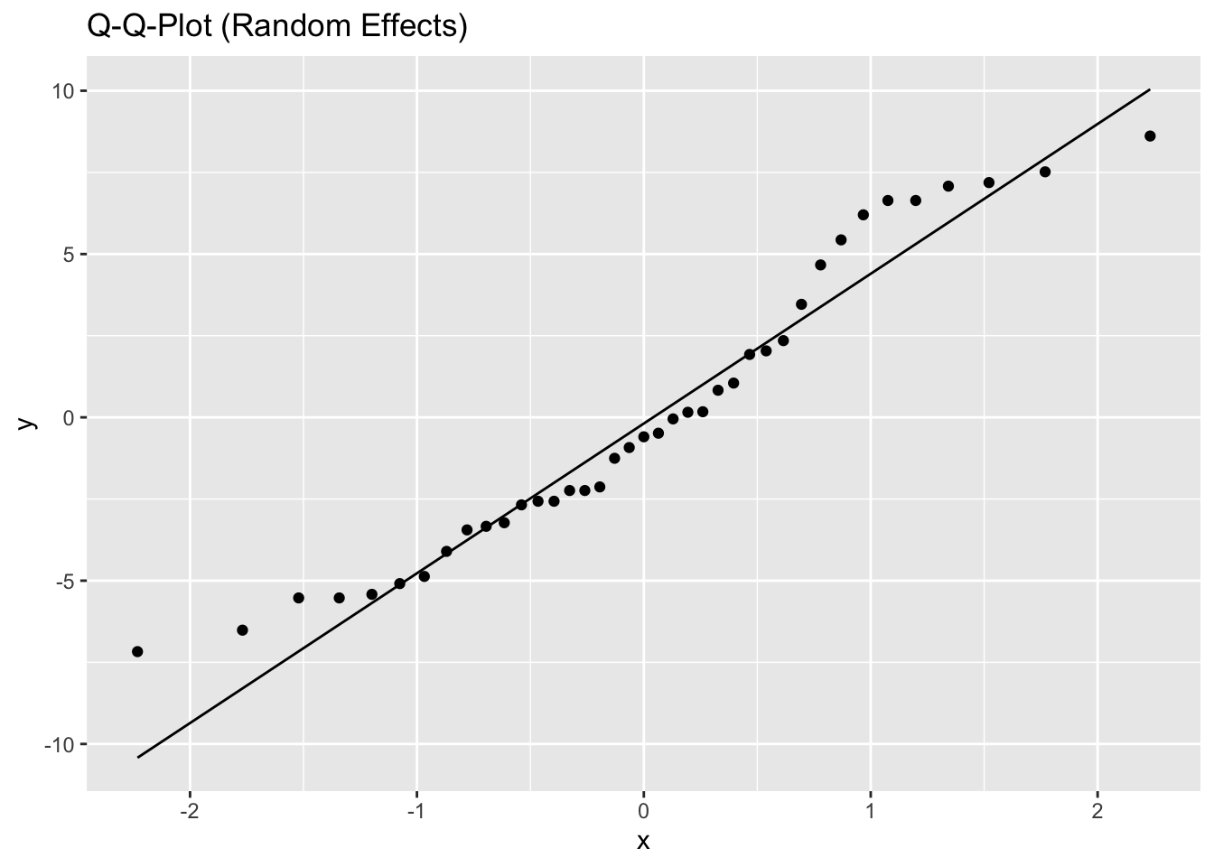
Inf_plots2(x, z)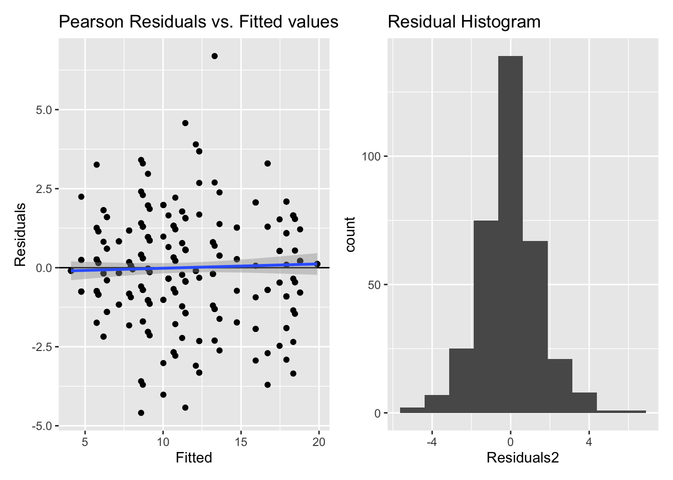
Inf_plots3(x, z, value, "identity")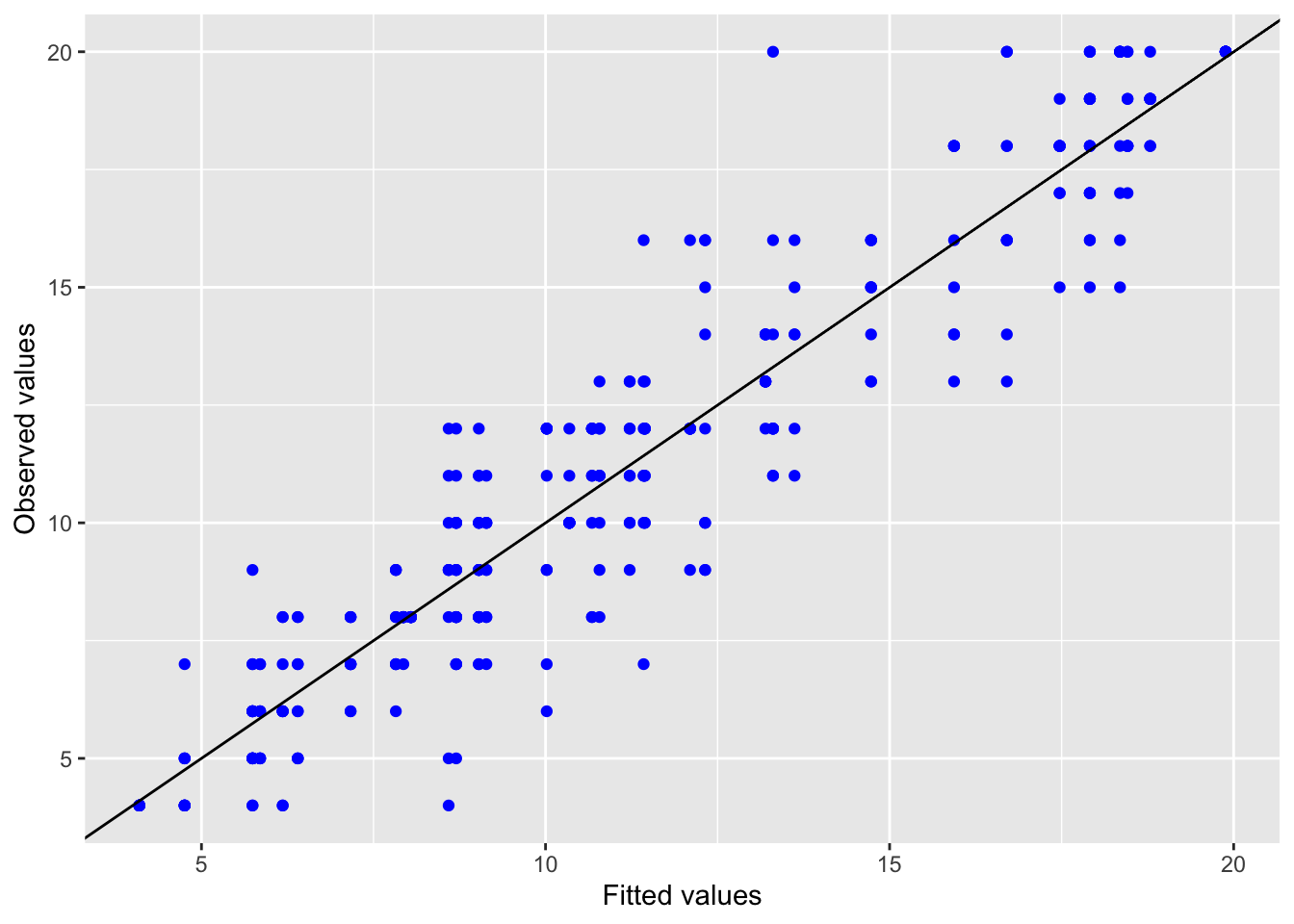
Inf_plots1(x, z)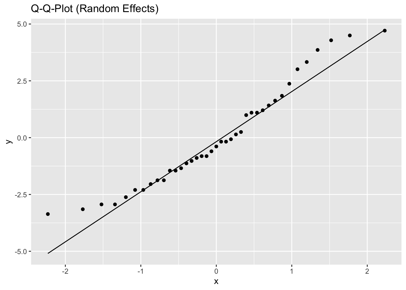
Inf_plots2(x, z)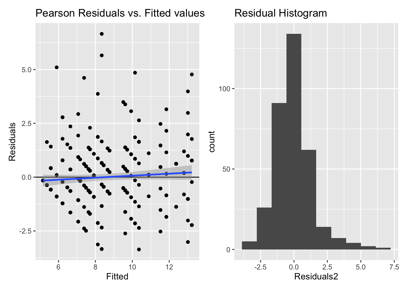
Inf_plots3(x, z, value, "identity")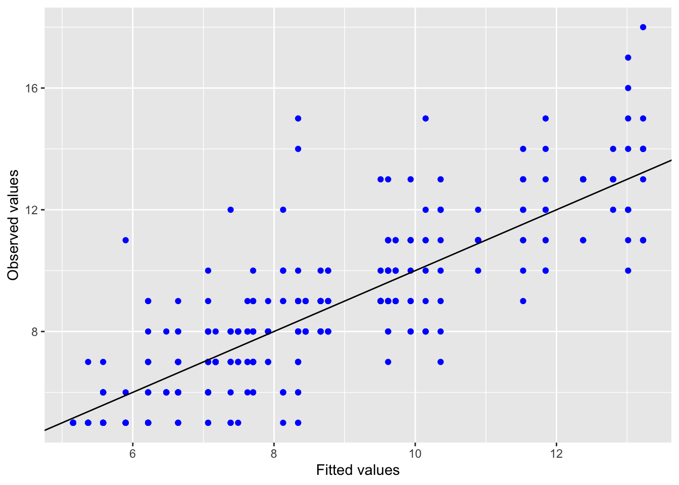
5.3.2 Hypothesis 4
\(H4\): LEBA scores vary over time within participants
For this hypothesis, only the malaysian data is used, as specified in the preregistration document.
bootstraps <- 10^4

leba_metrics_H4 <-
leba_metrics %>%
  mutate(data = list(data %>% filter(site == "malaysia")))

boot_plot <- function(data) {
  data %>%
  ggplot(aes(x = CI95lower/(1/3))) +
  geom_histogram(aes(fill = CI95lower/(1/3) >= 0.5), binwidth = 1, col = "white", alpha = 0.75) +
  scale_x_continuous(breaks = c(0:10)) +
  theme_void() +
  labs(x = "lower CI: Number of varying answers", y = "Frequency")+
  theme(axis.text = element_text(),
        legend.position = "none",
        axis.title.x = element_text(),
        panel.grid.major.y = element_line(colour = "grey80")) +
  scale_y_continuous(labels = scales::label_percent(scale = 100/19),
                     breaks = c(0, 50/100*19, 25/100*19, 75/100*19, 100/100*19))+
  coord_cartesian(ylim = c(0, 100/100*19))
}

leba_metrics_H4 <-
  leba_metrics_H4 %>%
  rowwise() %>%
  mutate(bootstrap =
           list(data %>%
               select(Id, value) %>%
               mutate(value = as.numeric(value)) %>%
               expand_grid(bootstrap = seq(bootstraps)) %>%
               group_by(Id, bootstrap) %>%
               slice_sample(prop = 1, replace = TRUE) %>%
               summarize(sd = stats::sd(value), .groups = "drop_last") %>%
               summarize(
                 mean_sd = mean(sd),
                 CI95lower = quantile(sd, 0.025),
                 CI95_upper = quantile(sd, 0.975),
                 .groups = "drop_last"
               ) %>%
               mutate(significant = ifelse(CI95lower == 0, FALSE, TRUE)) %>%
               summarize(
                 percent_significant = mean(significant),
                 plot = list(tibble(CI95lower) %>% boot_plot())
               )
           )
         )

labels_leba <-
var_label(leba_data_combined)[-c(1:3)] %>% enframe() %>% unnest(value)

leba_results_H4 <-
  leba_metrics_H4 %>%
  unnest(bootstrap) %>%
  select(-data) %>%
  left_join(labels_leba, by = c("metric" = "name")) %>%
  rename(question = value) %>%
  group_by(quartile =
             cut(
               percent_significant,
               breaks = c(-0.1, 0.25, 0.5, 0.75, 1.1),
               labels =
                 paste(
                   "stable over time in",
                   c("75-100%", "50-75%", "25-50%", "25-0%"),
                   "of participants"
                 )
             ))

leba_results_H4 %>%
  relocate(question, .before = 1) %>%
  arrange(percent_significant) %>%
  gt() %>%
  text_transform(
    locations = cells_body(columns = plot),
    fn = function(x)
      leba_results_H4$plot %>% ggplot_image(height = px(200))
  ) %>%
  fmt_percent(columns = percent_significant) %>%
  cols_label(plot = "",
             percent_significant = "Participants with significant variation",
             question = "Item/Factor",
             metric = "Metric code") %>%
  cols_align(align = "center", columns = -question) %>%
  tab_footnote(
    paste(
      "based on",
      bootstraps,
      "bootstraps of individual participants answers across the four weeks of data collection. If the lower threshold for a 95% confidence interval is above 0, the participant is considered to have significant variation in their answers."
    ),
    locations = cells_column_labels(columns = "percent_significant")
  ) %>%
  tab_header(title = "Model Results for Hypothesis 4") %>%
  tab_style(
    style = cell_text(weight = "bold"),
    locations = list(cells_column_labels(), cells_stub())
)| Model Results for Hypothesis 4 | |||
|---|---|---|---|
| Item/Factor | Metric code | Participants with significant variation1 | |
| stable over time in 75-100% of participants | |||
| I wear blue-filtering, orange-tinted, and/or red-tinted glasses within 1 hour before attempting to fall asleep | leba_F1_03 | 0.00% |  |
| I wear blue-filtering, orange-tinted, and/or red-tinted glasses indoors during the day | leba_F1_01 | 5.26% |  |
| I look at my smartwatch within 1 hour before attempting to fall asleep | leba_F3_13 | 5.26% |  |
| I look at my smartwatch when I wake up at night | leba_F3_14 | 5.26% |  |
| I wear blue-filtering, orange-tinted, and/or red-tinted glasses outdoors during the day | leba_F1_02 | 10.53% |  |
| I go for a walk or exercise outside within 2 hours after waking up | leba_F2_09 | 10.53% |  |
| I use my mobile phone within 1 hour before attempting to fall asleep | leba_F3_10 | 10.53% | |
| I use an alarm with a dawn simulation light | leba_F5_22 | 10.53% |  |
| Wearing blue light filtering glasses indoors and outdoors | leba_F1 | 10.53% | |
| I use tunable lights to create a healthy light environment | leba_F5_19 | 15.79% | |
| I use a desk lamp when I do focused work | leba_F5_21 | 15.79% | |
| stable over time in 50-75% of participants | |||
| I use a blue-filter app on my computer screen within 1 hour before attempting to fall asleep | leba_F4_16 | 26.32% |  |
| I spend between 30 minutes and 1 hour per day (in total) outside | leba_F2_05 | 31.58% | |
| I spend between 1 and 3 hours per day (in total) outside | leba_F2_06 | 31.58% | |
| I spend more than 3 hours per day (in total) outside | leba_F2_07 | 31.58% |  |
| I look at my mobile phone screen immediately after waking up | leba_F3_11 | 31.58% |  |
| I use LEDs to create a healthy light environment | leba_F5_20 | 31.58% |  |
| I spend as much time outside as possible | leba_F2_08 | 36.84% |  |
| I use as little light as possible when I get up during the night | leba_F4_17 | 36.84% |  |
| I spend 30 minutes or less per day (in total) outside | leba_F2_04 | 42.11% |  |
| I check my phone when I wake up at night | leba_F3_12 | 42.11% |  |
| I dim my mobile phone screen within 1 hour before attempting to fall asleep | leba_F4_15 | 42.11% | |
| I dim my computer screen within 1 hour before attempting to fall asleep | leba_F4_18 | 47.37% |  |
| I turn on the lights immediately after waking up | leba_F5_23 | 47.37% |  |
| stable over time in 25-50% of participants | |||
| Using phones and smartwatches in bed before sleep | leba_F3 | 73.68% |  |
| Using light in the morning and during daytime | leba_F5 | 73.68% |  |
| stable over time in 25-0% of participants | |||
| Spending time outdoors | leba_F2 | 84.21% |  |
| Controlling and using ambient light before bedtime | leba_F4 | 100.00% |  |
| 1 based on 10000 bootstraps of individual participants answers across the four weeks of data collection. If the lower threshold for a 95% confidence interval is above 0, the participant is considered to have significant variation in their answers. | |||
leba_H4_table <-
leba_results_H4 %>% select(metric, quartile) %>% nest(data = metric) %>%
  arrange(quartile) %>%
  mutate(data = map(data, ~.x %>% pull(metric) %>% paste(collapse = ", "))) %>%
  unnest(data) %>%
  mutate(data = str_replace_all(data, "leba_F", "Factor "),
         data = str_replace_all(data, "_", ": Item ")) %>%
  gt() %>%
  tab_style(
    style = cell_text(weight = "bold"),
    locations = cells_row_groups()
  ) %>%
  tab_options(column_labels.hidden = TRUE) %>%
  tab_header(title = "Hypothesis 4: Extent of stable LEBA items and factors over time")

leba_H4_table| Hypothesis 4: Extent of stable LEBA items and factors over time |
|---|
| stable over time in 75-100% of participants |
| Factor 1: Item 01, Factor 1: Item 02, Factor 1: Item 03, Factor 2: Item 09, Factor 3: Item 10, Factor 3: Item 13, Factor 3: Item 14, Factor 5: Item 19, Factor 5: Item 21, Factor 5: Item 22, Factor 1 |
| stable over time in 50-75% of participants |
| Factor 2: Item 04, Factor 2: Item 05, Factor 2: Item 06, Factor 2: Item 07, Factor 2: Item 08, Factor 3: Item 11, Factor 3: Item 12, Factor 4: Item 15, Factor 4: Item 16, Factor 4: Item 17, Factor 4: Item 18, Factor 5: Item 20, Factor 5: Item 23 |
| stable over time in 25-50% of participants |
| Factor 3, Factor 5 |
| stable over time in 25-0% of participants |
| Factor 2, Factor 4 |
leba_H4_table %>% gtsave("figures/Table_H4.png")

v1 <- leba_results_H4 %>% summarize(length = n())
As the two summary tables show, the majority of items is very stable over time in our sample. 24 items and factors don’t show significant variance in over half of participants. The factors are less stable over time and with the exception of Factor 1, all show variance in over 75% of participants. This is to be expected, as the factor calculation across items is more likely to show variance than individual items. The next section summarizes the average changes in and standard deviation of the LEBA metrics across the four weeks of data collection.
#average change
leba_changes <-
leba_metrics %>%
  mutate(data = list(data %>% filter(site == "malaysia")),
         data = list(data %>% mutate(value = as.numeric(value)) %>%
                       group_by(Id) %>%
                       summarize(sd = stats::sd(value), mean = mean(value),
                                 cv = sd/mean, .groups = "drop_last") %>%
                       summarize(mean_sd = mean(sd),
                                 mean_cv = mean(cv))))

leba_changes %>% unnest(data) %>% select(metric, mean_sd) %>%
  mutate(average_change = mean_sd/(1/3),
         average_change = average_change %>% round()) %>%
  left_join(labels_leba, by = c("metric" = "name")) %>%
  relocate(question = value, .before = 1) %>%
  gt() %>%
  fmt_number(columns = mean_sd, decimals = 2) %>%
    tab_style(
    style = cell_text(weight = "bold"),
    locations = cells_column_labels()
  ) %>%
  cols_label(
             question = "Item/Factor",
             metric = "Metric code",
             mean_sd = "SD",
             average_change = "Average change") %>%
  tab_footnote(
    "Average standard deviation across participants",
    locations = cells_column_labels(columns = "mean_sd")
  ) %>%
  tab_footnote(
        "Average change in scores total across the four weeks of data collection. A value of 1 indicates that across the 9 times of data collection, only once did a participant's score change by 1 point. A value of 2 indicates a score change once by 2 points, or two times by 1, and so forth.",
    locations = cells_column_labels(columns = "average_change")
  ) %>%
tab_header(title = "Average change in LEBA metrics across four weeks of data collection")| Average change in LEBA metrics across four weeks of data collection | |||
|---|---|---|---|
| Item/Factor | Metric code | SD1 | Average change2 |
| I wear blue-filtering, orange-tinted, and/or red-tinted glasses indoors during the day | leba_F1_01 | 0.10 | 0 |
| I wear blue-filtering, orange-tinted, and/or red-tinted glasses outdoors during the day | leba_F1_02 | 0.18 | 1 |
| I wear blue-filtering, orange-tinted, and/or red-tinted glasses within 1 hour before attempting to fall asleep | leba_F1_03 | 0.09 | 0 |
| I spend 30 minutes or less per day (in total) outside | leba_F2_04 | 0.57 | 2 |
| I spend between 30 minutes and 1 hour per day (in total) outside | leba_F2_05 | 0.54 | 2 |
| I spend between 1 and 3 hours per day (in total) outside | leba_F2_06 | 0.46 | 1 |
| I spend more than 3 hours per day (in total) outside | leba_F2_07 | 0.51 | 2 |
| I spend as much time outside as possible | leba_F2_08 | 0.39 | 1 |
| I go for a walk or exercise outside within 2 hours after waking up | leba_F2_09 | 0.24 | 1 |
| I use my mobile phone within 1 hour before attempting to fall asleep | leba_F3_10 | 0.27 | 1 |
| I look at my mobile phone screen immediately after waking up | leba_F3_11 | 0.46 | 1 |
| I check my phone when I wake up at night | leba_F3_12 | 0.57 | 2 |
| I look at my smartwatch within 1 hour before attempting to fall asleep | leba_F3_13 | 0.08 | 0 |
| I look at my smartwatch when I wake up at night | leba_F3_14 | 0.07 | 0 |
| I dim my mobile phone screen within 1 hour before attempting to fall asleep | leba_F4_15 | 0.62 | 2 |
| I use a blue-filter app on my computer screen within 1 hour before attempting to fall asleep | leba_F4_16 | 0.27 | 1 |
| I use as little light as possible when I get up during the night | leba_F4_17 | 0.70 | 2 |
| I dim my computer screen within 1 hour before attempting to fall asleep | leba_F4_18 | 0.55 | 2 |
| I use tunable lights to create a healthy light environment | leba_F5_19 | 0.28 | 1 |
| I use LEDs to create a healthy light environment | leba_F5_20 | 0.49 | 1 |
| I use a desk lamp when I do focused work | leba_F5_21 | 0.25 | 1 |
| I use an alarm with a dawn simulation light | leba_F5_22 | 0.19 | 1 |
| I turn on the lights immediately after waking up | leba_F5_23 | 0.54 | 2 |
| Wearing blue light filtering glasses indoors and outdoors | leba_F1 | 0.32 | 1 |
| Spending time outdoors | leba_F2 | 1.40 | 4 |
| Using phones and smartwatches in bed before sleep | leba_F3 | 1.03 | 3 |
| Controlling and using ambient light before bedtime | leba_F4 | 1.33 | 4 |
| Using light in the morning and during daytime | leba_F5 | 1.28 | 4 |
| 1 Average standard deviation across participants | |||
| 2 Average change in scores total across the four weeks of data collection. A value of 1 indicates that across the 9 times of data collection, only once did a participant's score change by 1 point. A value of 2 indicates a score change once by 2 points, or two times by 1, and so forth. | |||
5.4 Research Question 3
RQ 3 In general, how are light exposure and LEBA related and are there differences in this relationship between the two sites?
5.4.0.1 Metric calculation
Additional metrics need to be calculated:
- First time above threshold 250 lx mel EDI (FLiT250)
- First time above threshold 1000 lx mel EDI (FLiT1000)
- L5 without sleep period (night), i.e. day and evening (L5mde)
- L5 only night time (L5mn)
- Melanopic/photopic ratio (MPratio)
- Light exposure (dose of light) for melanopic EDI (LE)
- Spectral contribution to melanopic EDI (SCmelEDI) 1
p_adjustment <- append(
  p_adjustment,
  list(
  H5 = 2*84,
  H6 = 23+5
))

metrics <-
  rbind(
    metrics,
    data %>%
map(
  \(x) {
      #whole-day metrics
      whole_day <-
      x %>%
        group_by(Id, Day) %>%
        summarize(
          .groups = "drop",
          FLiT1000 =
            timing_above_threshold(
              MEDI, Datetime, "above", 1000, as.df = TRUE) %>%
            pull(first_timing_above_1000) %>% hms::as_hms() %>% as.numeric(),
          FLiT250 =
            timing_above_threshold(MEDI, Datetime, "above", 250, as.df = TRUE) %>%
            pull(first_timing_above_250) %>% hms::as_hms() %>% as.numeric(),
          MPratio = mean(MEDI, na.rm = TRUE)/mean(Photopic.lux, na.rm = TRUE),
          LE = sum(MEDI, na.rm = TRUE)/60,
          SCmelEDI = mean(MEDI, na.rm = TRUE)/753.35/
            mean(rowSums(across(starts_with("WL_")))*1000, na.rm = TRUE)
        ) %>%
        mutate(across(where(is.duration), as.numeric)) %>%
        pivot_longer(cols = -c(Id, Day), names_to = "metric")

      #part-day metrics
      part_day <-
        x %>%
        group_by(Id, Day, Night = Photoperiod == "night") %>%
        summarize(
          .groups = "drop",
          L5m =
            bright_dark_period(
                  MEDI, Datetime, "darkest", "5 hours", as.df = TRUE,
                  na.rm = TRUE
                  ) %>% pull(darkest_5h_mean) %>% log10()
        ) %>%
        pivot_longer(cols = -c(Id, Day, Night), names_to = "metric") %>%
        mutate(metric = case_when(
          metric == "L5m" & Night == TRUE ~ "L5mn",
          metric == "L5m" & Night == FALSE ~ "L5mde"
        ))

      whole_day %>%
        bind_rows(part_day)
    }
  ) %>%
  list_rbind(names_to = "site") %>%
  nest(data = -metric)
  )

#nest the datasets by site
metricsRQ3 <-
  metrics %>%
  rowwise() %>%
  mutate(data = list(data %>%
                       mutate(across(any_of("Day"), as_date))
                     )
         ) %>%
  unnest(data) %>%
  nest(data = -c(site, metric)) %>%
  nest(data = -site)

#select relevant metrics by question
metric_selection$H5 <-
  list(
    leba_F1_01 = c(),
    leba_F1_02 = c(),
    leba_F1_03 = c(),
    leba_F2_04 = c("M10m", "TAT250", "TAT1000", "PAT1000", "IV", "IS"),
    leba_F2_05 = c("M10m", "TAT250", "TAT1000", "PAT1000", "IV", "IS"),
    leba_F2_06 = c("M10m", "TAT250", "TAT1000", "PAT1000", "IV", "IS"),
    leba_F2_07 = c("M10m", "TAT250", "TAT1000", "PAT1000", "IV", "IS"),
    leba_F2_08 = c("M10m", "TAT250", "TAT1000", "PAT1000", "IV", "IS"),
    leba_F2_09 = c("FLiT1000", "IV", "IS"),
    leba_F3_10 = c("LLiT10", "LLiT250", "L5mn", "IV", "IS"),
    leba_F3_11 = c("FLiT250", "IV", "IS"),
    leba_F3_12 = c("L5m", "IV", "IS"),
    leba_F3_13 = c("LLiT10", "LLiT250", "L5mn", "IV", "IS"),
    leba_F3_14 = c("L5m", "IV", "IS"),
    leba_F4_15 = c("LLiT10", "LLiT250", "L5mde", "IV", "IS"),
    leba_F4_16 = c("LLiT10", "LLiT250", "L5mde", "IV", "IS"),
    leba_F4_17 = c("L5m", "L5mn", "IV", "IS"),
    leba_F4_18 = c("LLiT10", "LLiT250", "L5mde", "IV", "IS"),
    leba_F5_19 = c("IV", "IS", "L5mn", "L5mde", "M10m"),
    leba_F5_20 = c("LE", "SCmelEDI", "MPratio"),
    leba_F5_21 = c("LE"),
    leba_F5_22 = c("SCmelEDI", "FLiT10", "FLiT250"),
    leba_F5_23 = c("SCmelEDI", "FLiT10", "FLiT250")
  )

#transform relevant metrics to a table of metrics
metric_selectionH5 <-
metric_selection$H5 %>%
  enframe() %>%
  unnest(value) %>%
  mutate(hypothesised = TRUE)
5.4.1 Hypothesis 5
\(H5\): LEBA items correlate with preselected light-logger derived light exposure variables.
Due to how the LEBA questions were phrased, different timespan comparisons are needed. For Malaysia, only the last instance is used and average metric values are calculated from daily data. For Switzerland, respective time periods are compared to one another, i.e. a LEBA period of 4 days is compared to the light exposure metrics from the same 4 days, and averaged over those days for a one-to-one comparison.
#collect the light exposure data for malaysia
metrics_H5_malaysia <-
  metricsRQ3 %>%
  filter(site == "malaysia") %>%
  unnest(data) %>%
  select(-site) %>%
  filter(metric != "mean")

#average values across all days
metrics_H5_malaysia <-
  metrics_H5_malaysia %>%
  rowwise() %>%
  mutate(data = list(data %>%
                       group_by(Id) %>%
                       summarize(value = mean(value, na.rm = TRUE), .groups = "drop")
  )
  )

#collect the appropriate day for the LEBA data
leba_H5_malaysia <-
  leba_data_combined %>% filter(site == "malaysia", Day ==31) %>%
  select(-Datetime, -site, -Day) %>%
    mutate(across(-Id, as.numeric)) %>%
  pivot_longer(cols = -Id, names_to = "leba", values_to = "leba_values")

#join the data
leba_light_H5_malaysia <-
metrics_H5_malaysia %>%
  unnest(data) %>%
  rename(metric_value = value) %>%
  left_join(leba_H5_malaysia, by = "Id",
            relationship = "many-to-many") %>%
  select(-Id) %>%
  drop_na()

#calculate correlations
corr_malaysia <-
  leba_light_H5_malaysia %>%
    group_by(metric, leba) %>%
    summarize(
      correlation = cor(metric_value, leba_values, method = "spearman"),
              p_value = cor.test(metric_value, leba_values)$p.value,
              p_value_adjusted =p.adjust(p_value, method = "fdr",
                                         n = p_adjustment$H5),
              significant = p_value <= 0.05,
              significant_adjusted = p_value_adjusted <= 0.05,
              .groups = "drop") %>%
  mutate(
    question = leba_questions[leba],
    factor = leba_factors[leba],
    question = ifelse(is.na(question), factor, question),
    .before = 1) %>%
  fill(factor) %>%
  left_join(metric_selectionH5, by = c("metric" = "value", "leba" = "name")) %>%
  mutate(hypothesised = ifelse(is.na(hypothesised), FALSE, hypothesised),
         coloring = case_when(
           significant_adjusted & hypothesised ~ "Hypothesised and significant",
           significant & hypothesised ~ "Hypothesised and (unadjusted) significant",
           significant & !hypothesised ~ "(unadjusted) Significant",
           !significant_adjusted & hypothesised ~ "Hypothesised",
           TRUE ~ "None"
         ) %>% factor(levels = c("Hypothesised and significant", "Hypothesised and (unadjusted) significant", "(unadjusted) Significant", "Hypothesised", "None")
         )
         ) %>%
    mutate(
    leba = leba %>%
        str_remove("leba_") %>%
        str_replace("_", ", ") %>%
        str_replace("(F[:digit:])$", "\\1 (overall)")
  )

colors_H5 <- c("gold", "orange", "white", "red", "grey")


#display the results
corr_plot_malaysia <-
corr_malaysia %>%
  ggplot(aes(x = metric, y = (leba %>% factor() %>% fct_rev()), fill = abs(correlation), col = coloring)) +
  geom_blank()+
  geom_tile(data = corr_malaysia %>% filter(coloring != "None"), linewidth = 0.25) +
  geom_text(
    aes(label =
          paste(
            paste("c=",round(correlation, 2)),
            p_value %>% style_pvalue(prepend_p = TRUE),
            sep = "\n")
        ),
    fontface = "bold",
    size = 1.8) +
  coord_fixed() +
  scale_fill_viridis_c(limits = c(0,1))+
  scale_color_manual(values = colors_H5, drop = FALSE)+
  labs(y = "LEBA questions and factors", x = "Metrics", color = "Relevance",
       fill = "(abs) Correlation", subtitle = "Malaysia")+
  theme(axis.text.x = element_text(angle = 90, hjust = 1),
        plot.subtitle = element_text(color = pal_jco()(1)))

corr_plot_malaysia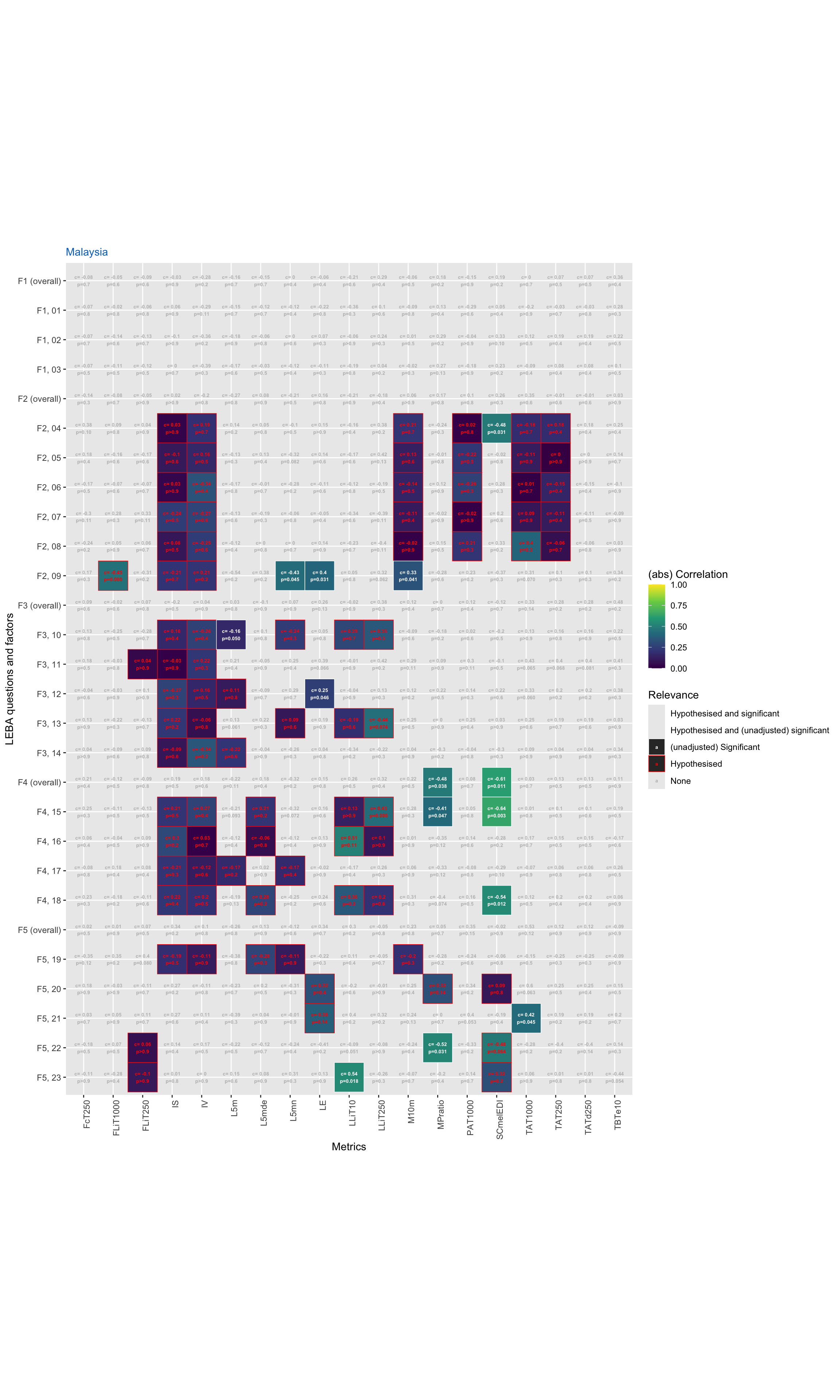
To combine relevant metrics with LEBA questionnaires, Metric days will be associated with days of LEBA questionnaires and previous days up until the previous collection point.
#collect the light exposure data for Switzerland
metrics_H5_switzerland <-
  metricsRQ3 %>%
  filter(site == "switzerland") %>%
  unnest(data) %>%
  select(-site) %>%
  filter(metric != "mean") %>%
  filter(metric != "IS")
  #we have to remove IS for now, as it has to be computed for each section for Switzerland

#collect the appropriate day for the LEBA data
leba_H5_switzerland <-
  leba_data_combined %>% filter(site == "switzerland") %>%
  mutate(
    leba_col_period = Day,
    Day = date(Datetime)) %>%
  select(-Datetime, -site) %>%
    mutate(across(-c(Id, Day, leba_col_period), as.numeric))

#average values across collection days
metrics_H5_switzerland <-
metrics_H5_switzerland %>%
  rowwise() %>%
  mutate(data = list(
    data %>%
  full_join(leba_H5_switzerland, by = c("Id", "Day")) %>%
  arrange(Id, Day) %>%
  fill(starts_with("leba_"), .direction = "up") %>%
  drop_na(value) %>%
  rename(col_period = leba_col_period) %>%
  pivot_longer(cols = starts_with("leba_"), names_to = "leba", values_to = "leba_values") %>%
  group_by(Id, col_period) %>%
  summarize(
    value = mean(value, na.rm = TRUE), .groups = "drop"
  )
  ))

#calculating IS for Switzerland for each section
data_collection_switzerland <-
leba_H5_switzerland %>%
  group_by(Id,  Day, leba_col_period) %>%
  summarize(.groups = "drop")

metrics_H5_switzerland_IS <-
data$switzerland %>%
  full_join(data_collection_switzerland, by = c("Id", "Day")) %>%
  arrange(Id, Day) %>%
  fill(starts_with("leba_"), .direction = "up") %>%
  group_by(Id, leba_col_period) %>%
  summarize(
    IS = interdaily_stability(MEDI, Datetime, na.rm = TRUE),
    .groups = "drop"
  ) %>%
  rename(col_period = leba_col_period) %>%
  pivot_longer(cols = IS, names_to = "metric", values_to = "value") %>%
  drop_na(value) %>%
  nest(data = -metric)

metrics_H5_switzerland <-
  rbind(metrics_H5_switzerland,
        metrics_H5_switzerland_IS)

#transform the LEBA data to the appropriate format
leba_H5_switzerland <-
  leba_H5_switzerland %>%
  pivot_longer(cols = -c(Id, Day, leba_col_period),
               names_to = "leba", values_to = "leba_values")

#join the data
leba_light_H5_switzerland <-
metrics_H5_switzerland %>%
  unnest(data) %>%
  rename(metric_value = value) %>%
  left_join(leba_H5_switzerland, by = c("Id", "col_period" = "leba_col_period"),
            relationship = "many-to-many") %>%
  select(-Id) %>%
  drop_na()


#calculate correlations
corr_switzerland <-
  leba_light_H5_switzerland %>%
    group_by(metric, leba) %>%
    summarize(
      correlation = cor(metric_value, leba_values, method = "spearman"),
              p_value = cor.test(metric_value, leba_values)$p.value,
              p_value_adjusted =p.adjust(p_value, method = "fdr",
                                         n = p_adjustment$H5),
              significant = p_value <= 0.05,
              significant_adjusted = p_value_adjusted <= 0.05,
              .groups = "drop") %>%
  mutate(
    question = leba_questions[leba],
    factor = leba_factors[leba],
    question = ifelse(is.na(question), factor, question),
    .before = 1) %>%
  fill(factor) %>%
  left_join(metric_selectionH5, by = c("metric" = "value", "leba" = "name")) %>%
  mutate(hypothesised = ifelse(is.na(hypothesised), FALSE, hypothesised),
         coloring = case_when(
           significant_adjusted & hypothesised ~ "Hypothesised and significant",
           significant & hypothesised ~ "Hypothesised and (unadjusted) significant",
           significant & !hypothesised ~ "(unadjusted) Significant",
           !significant_adjusted & hypothesised ~ "Hypothesised",
           TRUE ~ "None"
         ) %>% factor(levels = c("Hypothesised and significant", "Hypothesised and (unadjusted) significant", "(unadjusted) Significant", "Hypothesised", "None")
         )) %>%
      mutate(
    leba = leba %>%
        str_remove("leba_") %>%
        str_replace("_", ", ") %>%
        str_replace("(F[:digit:])$", "\\1 (overall)")
  )


#display the results
corr_plot_switzerland <-
corr_switzerland %>%
  ggplot(aes(x = metric, y = (leba %>% factor() %>% fct_rev()), fill = abs(correlation), col = coloring)) +
  geom_tile(data = corr_switzerland %>% filter(coloring != "None"), linewidth = 0.25) +
  geom_text(
    aes(label =
          paste(
            paste("c=",round(correlation, 2)),
            p_value %>% style_pvalue(prepend_p = TRUE),
            sep = "\n")
        ),
    size = 1.8,
    fontface = "bold") +
  coord_fixed() +
  scale_fill_viridis_c(limits = c(0,1))+
  scale_color_manual(values = colors_H5, drop = FALSE)+
  labs(y = "LEBA questions and factors", x = "Metrics", color = "Relevance",
       fill = "(abs) Correlation", subtitle = "Switzerland")+
  theme(axis.text.x = element_text(angle = 90, hjust = 1),
        plot.subtitle = element_text(color = pal_jco()(2)[2]))

corr_plot_switzerland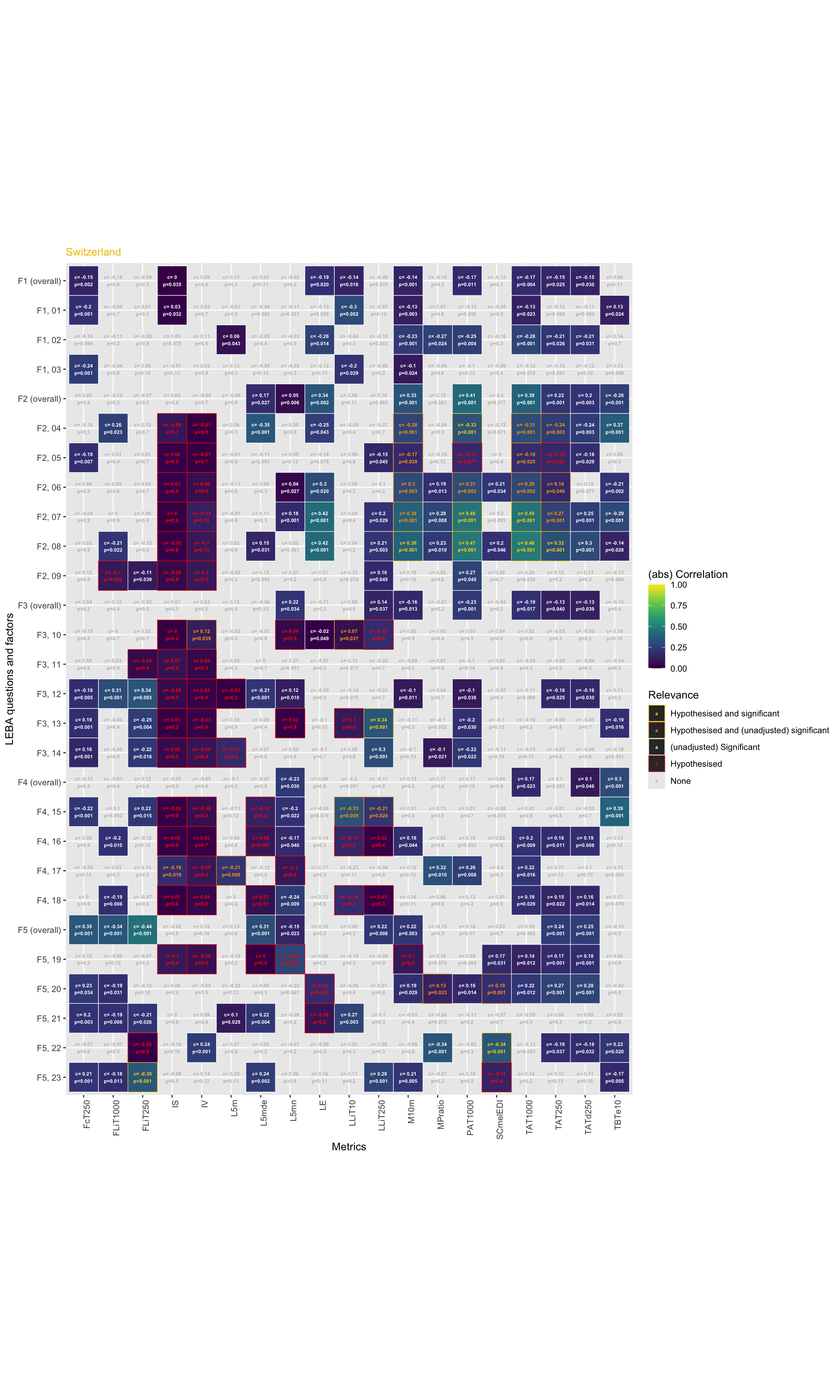
#visualization
(corr_plot_malaysia + theme(legend.position = "none")) + corr_plot_switzerland + plot_layout(guides = "collect")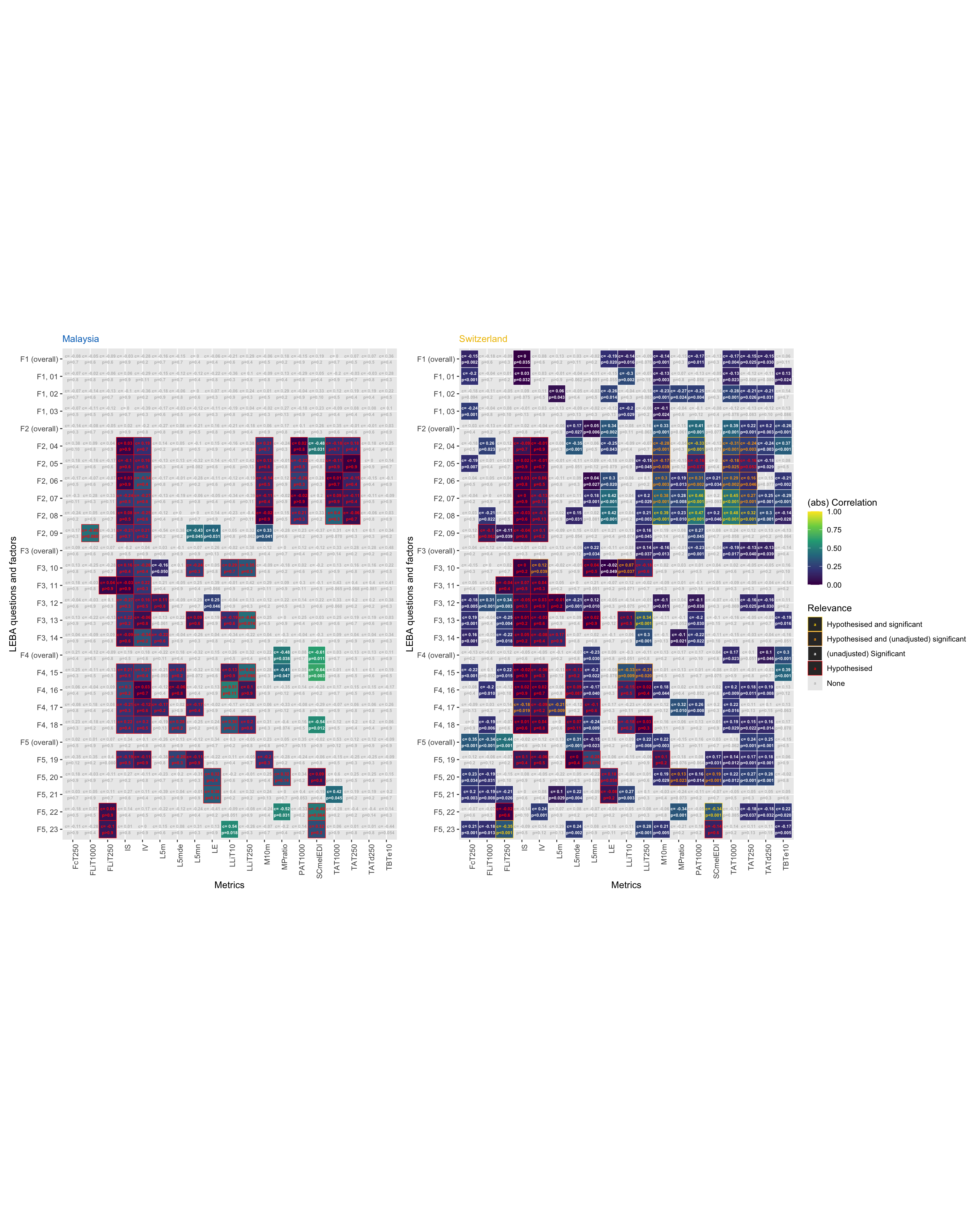
corr_results <- list_rbind(
  list(malaysia = corr_malaysia,
       switzerland = corr_switzerland),
  names_to = "site")

#summary of restuls
corr_results %>%
  select(site, coloring) %>%
  tbl_summary(by = site,
              label = list(coloring ~ "Summary of correlation matrices")) %>%
  as_gt() %>%
gt::tab_header(title = "Results for Hypothesis 5")| Results for Hypothesis 5 | ||
|---|---|---|
| Characteristic | malaysia N = 5321 |
switzerland N = 5321 |
| Summary of correlation matrices | ||
| Hypothesised and significant | 0 (0%) | 10 (1.9%) |
| Hypothesised and (unadjusted) significant | 0 (0%) | 19 (3.6%) |
| (unadjusted) Significant | 14 (2.6%) | 150 (28%) |
| Hypothesised | 84 (16%) | 55 (10%) |
| None | 434 (82%) | 298 (56%) |
| 1 n (%) | ||
corr_results %>% group_by(site, coloring) %>% summarize(n = n(), mean_cor = mean(abs(correlation)), max_cor = max(abs(correlation))) %>%
  gt() %>%
  tab_header("Summary of correlation coefficients by type, Hypothesis 5") %>%
  tab_footnote(
    "Mean correlation is the average of the absolute correlation coefficients",
    locations = cells_column_labels(columns = "mean_cor")
  ) %>%
  tab_footnote(
    "Max correlation is the highest absolute correlation coefficient",
    locations = cells_column_labels(columns = "max_cor")
  ) %>%
#make col labels and row labels bold
  tab_style(
    style = list(
      cell_text(weight = "bold")
    ),
    locations = list(cells_column_labels(), cells_row_groups())
  ) %>%
  cols_label(
    coloring = "",
    mean_cor = "Mean correlation",
    max_cor = "Max correlation"
  ) %>%
  fmt_number(
    columns = c(mean_cor, max_cor),
    decimals = 2
  ) %>%
  text_transform(str_to_title, locations = cells_row_groups()) %>%
cols_align(align = "left", columns = coloring)| Summary of correlation coefficients by type, Hypothesis 5 | |||
|---|---|---|---|
| n | Mean correlation1 | Max correlation2 | |
| Malaysia | |||
| (unadjusted) Significant | 14 | 0.44 | 0.64 |
| Hypothesised | 84 | 0.19 | 0.51 |
| None | 434 | 0.17 | 0.60 |
| Switzerland | |||
| Hypothesised and significant | 10 | 0.39 | 0.48 |
| Hypothesised and (unadjusted) significant | 19 | 0.23 | 0.38 |
| (unadjusted) Significant | 150 | 0.21 | 0.44 |
| Hypothesised | 55 | 0.07 | 0.28 |
| None | 298 | 0.09 | 0.30 |
| 1 Mean correlation is the average of the absolute correlation coefficients | |||
| 2 Max correlation is the highest absolute correlation coefficient | |||
interpretation <-
  c("The more often 30 minutes or less are spent outside, the shorter the period above 1000 lx",
    "The more often >3 hours per day are spent outside, the longer the period above 1000 lx",
    "The more often > 3 hours per day are spent outside, the higher the time above 1000 lx",
    "The more spend time outside as possible, the brighter the brightest 10 hours (mean)",
    "The more spend time outside as possible, the longer the period above 1000 lx",
    "The more spend time outside as possible, the higher the time above 1000 lx",
    "The more spend time outside as possible, the higher the time above 250 lx",
    "The more often smartwatches are looked at within 1h before attempting to fall asleep, the later the last time above 250 lx",
    "The more an alarm with a dawn simulation light is used, the warmer the light colour temperature",
    "The more often the lights are turned on immediately after waking up, the earlier the first time above 250 lx"
    )

table <-
corr_results %>% filter(significant_adjusted) %>%
  select(-c(p_value, significant, significant_adjusted, factor, coloring)) %>%
  mutate(across(starts_with("p_value"), style_pvalue),
         correlation = correlation %>% round(2)) %>%
  arrange(leba) %>%
  filter(hypothesised) %>%
  gt() %>%
  cols_hide(hypothesised) %>%
  tab_header("Summary of significant results for Hypothesis 5") %>%
    tab_footnote(
      paste("p-values are adjusted for multiple comparisons using the false-discovery-rate for n=", p_adjustment$H5, "comparisons"),
      locations = cells_column_labels(columns = "p_value_adjusted")
    ) %>%
    tab_footnote(
      "Indication whether this specific combination was hypothesised in the preregistration document",
      locations = cells_column_labels(columns = "hypothesised")
    ) %>%
    tab_footnote(
      "Spearman correlation coefficient between the metric and the LEBA question/factor",
      locations = cells_column_labels(columns = "correlation")
    ) %>%
  cols_label(
    site = "Site",
    question = "Question/Factor",
    leba = "LEBA item",
    correlation = "Correlation coefficient",
    p_value_adjusted = "p-value",
    metric = "Metric"
  ) %>%
  cols_add(Interpretation = interpretation) %>%
  fmt(columns = leba, fns = \(x) x %>% str_remove("leba_") %>%
        str_replace("_", ", "))

  gtsave(table, "figures/Table_2.png", vwidth = 1100)
  gtsave(table, "figures/Table_2.docx")
The results clearly show that there are strong correlations between certain light exposure metrics and answers to the LEBA questionnaire, but only in the Swiss dataset. After adjustment for multiple comparisons, none of the correlations in the Malaysian dataset remained significant. Interestingly, the average (absolute) correlation is stronger in the Malaysia site compared to the Switzerland site, indicating a higher variance in either light exposure metrics or LEBA answers in the Malaysia dataset, compared to Switzerland. For the Swiss dataset, 10 of the hypothesised correlations proved to be significant, with on average medium effect size (Cohen 1988, 1992). For exploratory reasons, unadjusted significance levels are left in the matrices.
5.4.2 Hypothesis 6
\(H6\): There is a difference between Malaysia and Switzerland on how well light-logger derived light exposure variables correlate with subjective LEBA items.
The preregistration document specifies a generalized mixed model approach to test this hypothesis. As the speficied formula does not lead to to the stated number of models, i.e. 23+5, and also does not provide an overall overview of whether selected light exposure metrics correlate with LEBA items and factors, we provide an alternative approach by modelling the dependency of correlation coefficients on site, which gives a more condensed output and uses a linear model. The stricter analysis is still included in the analysis documentation.
leba_light_H6 <-
corr_results %>%
  filter(hypothesised) %>%
  nest(data = -c(leba, question, factor)) %>%
  arrange(leba)

#hypothesis formulas
formula_H6 <- correlation ~ site
formula_H0 <- correlation ~ 1

inference_H6 <-
  leba_light_H6 %>%
  mutate(formula_H1 = c(formula_H6),
         formula_H0 = c(formula_H0),
         type = "lm",
         family = list(gaussian()),
         metric = leba
         )


inference_H6 <-
inference_H6 %>%
  rowwise() %>%
  mutate(model = list(lm(data = data, formula = formula_H1)),
         model0 = list(lm(data = data, formula = formula_H0)),
         comparison = list(anova(model, model0)),
        p.value_adj = comparison %>% tidy() %>% pull(p.value) %>% .[2] %>%
        p.adjust(method = "fdr", n = p_adjustment$H6),
      significant = p.value_adj <= 0.05,
      summary = list(
        switch(significant+1,
               tidy(model0),
               tidy(model)))
  ) %>%
  drop_na() %>%
  rowwise() %>%
  mutate(
    table = list(
        tibble(
          metric = metric,
          p.value =
            p.value_adj %>%
            style_pvalue() %>%
            {ifelse(significant, paste0("**", ., "**"),.)},
          summary %>%
            mutate(estimate = estimate) %>%
            select(term, estimate) %>%
            mutate(term = str_remove_all(term, "\\(|\\)|site")) %>%
            pivot_wider(names_from = term, values_from = estimate)
        ) %>%
          mutate(malaysia = if(exists("switzerland")) 0 else NA, .after = Intercept)
    )
  )

Inference_Table_H6 <-
inference_H6 %>%
  mutate(metric = leba) %>%
Inference_Table(p_adjustment = p_adjustment$H6, value = correlation) %>%
  fmt_number("Intercept", decimals = 2) %>%
  fmt_number("switzerland", decimals = 2) %>%
  cols_align(align = "center", columns = "p.value") %>%
  tab_header(title = "Model Results for Hypothesis 6")

Inference_Table_H6| Model Results for Hypothesis 6 | |||||
|---|---|---|---|---|---|
| p-value1 | Intercept |
Site coefficients
|
|||
| Malaysia | Switzerland | ||||
| F2, 04 | 0.2 | −0.07 | — | — |  |
| F2, 05 | 0.9
|
−0.07 | — | — |  |
| F2, 06 | 0.048 | −0.14 | 0 | 0.33 |  |
| F2, 07 | 0.4 | 0.06 | — | — |  |
| F2, 08 | 0.9
|
0.16 | — | — |  |
| F2, 09 | 0.9
|
−0.08 | — | — |  |
| F3, 10 | 0.9
|
0.03 | — | — |  |
| F3, 11 | 0.9
|
0.05 | — | — |  |
| F3, 12 | 0.9
|
−0.01 | — | — |  |
| F3, 13 | 0.9
|
0.01 | — | — |  |
| F3, 14 | 0.9
|
−0.08 | — | — |  |
| F4, 15 | 0.020 | 0.25 | 0 | −0.40 |  |
| F4, 16 | 0.9
|
0.09 | — | — |  |
| F4, 17 | 0.9
|
−0.16 | — | — |  |
| F4, 18 | 0.038 | 0.25 | 0 | −0.26 |  |
| F5, 19 | 0.9
|
−0.10 | — | — |  |
| F5, 20 | 0.9
|
0.21 | — | — |  |
| F5, 22 | 0.9
|
−0.20 | — | — |  |
| F5, 23 | 0.9
|
−0.07 | — | — |  |
| 1 p-values are adjusted for multiple comparisons using the false-discovery-rate for n= 28 comparisons | |||||
Inference_Table_H6 %>% gtsave("figures/Table_H6.png")

v1 <- inference_H6 %>% filter(significant) %>% pull(question)
#join the data
leba_light_H6_malaysia <-
metrics_H5_malaysia %>%
unnest(data) %>%
rename(metric_value = value) %>%
left_join(leba_H5_malaysia, by = "Id",
relationship = "many-to-many") %>%
drop_na()
#join the data
leba_light_H6_switzerland <-
metrics_H5_switzerland %>%
unnest(data) %>%
rename(metric_value = value) %>%
left_join(leba_H5_switzerland, by = c("Id", "col_period" = "leba_col_period"),
relationship = "many-to-many") %>%
drop_na()
#create a combined dataset with metrics and LEBA items
light_leba_combined <-
list_rbind(
list(malaysia = leba_light_H6_malaysia,
switzerland = leba_light_H6_switzerland ),
names_to = "site") %>%
select(-col_period, -Day) %>%
nest(data = -c(metric, leba)) %>%
left_join(metric_selectionH5, by = c("metric" = "value", "leba" = "name")) %>%
filter(hypothesised) %>%
select(-hypothesised)
#hypothesis formulas
formula_H6 <- metric_value ~ site*leba_values + (1|site:Id)
formula_H0 <- metric_value ~ leba_values + (1|site:Id)
lmer <- lme4::lmer
inference_H6.2 <-
light_leba_combined %>%
mutate(formula_H1 = c(formula_H6),
formula_H0 = c(formula_H0),
type = "lmer",
family = list(gaussian())
)
inference_H6.2 <-
inference_H6.2 %>%
inference_summary2(p_adjustment = p_adjustment$H6)
inference_H6.2 %>%
rowwise() %>%
mutate(metric_leba = paste(metric, leba %>% str_remove("leba_") %>%
str_replace("_", ", "), sep = " & "),
table = list(table %>% mutate(metric = metric_leba))) %>%
Inference_Table(p_adjustment = p_adjustment$H6, value = metric_value) %>%
fmt_number("Intercept", decimals = 2) %>%
fmt_number("switzerland", decimals = 2) %>%
cols_align(align = "center", columns = "p.value") %>%
tab_header(title = "Model Results for Hypothesis 6")| Model Results for Hypothesis 6 | |||||||
|---|---|---|---|---|---|---|---|
| p-value1 | Intercept |
Site coefficients
|
leba_values | switzerland:leba_values | |||
| Malaysia | Switzerland | ||||||
| TAT250 & F2, 04 | 0.072 | 12,390.09 | — | — | -9.040267e+02 | — |  |
| TAT250 & F2, 05 | 0.052 | 9,998.34 | — | — | 9.516650e+00 | — | |
| TAT250 & F2, 06 | 0.027 | 7,221.81 | 0 | 3,344.20 | -4.665635e+02 | 1.056576e+03 | |
| TAT250 & F2, 07 | 0.004 | 6,932.53 | 0 | 1,784.68 | -4.005614e+02 | 1.889049e+03 | |
| TAT250 & F2, 08 | 0.041 | 6,142.27 | 0 | 2,323.64 | -1.594537e+02 | 1.509960e+03 | |
| TAT1000 & F2, 04 | 0.9
|
7,535.08 | — | — | -9.475831e+02 | — |  |
| TAT1000 & F2, 05 | 0.5 | 5,638.13 | — | — | -1.709208e+02 | — | |
| TAT1000 & F2, 06 | 0.2 | 3,547.15 | — | — | 5.489428e+02 | — | |
| TAT1000 & F2, 07 | 0.004 | 2,827.73 | 0 | −656.85 | -4.446896e+01 | 1.748464e+03 | |
| TAT1000 & F2, 08 | 0.3 | 1,404.46 | — | — | 1.433454e+03 | — | |
| PAT1000 & F2, 04 | 0.9
|
2,309.81 | — | — | -3.297124e+02 | — |  |
| PAT1000 & F2, 05 | 0.9
|
1,869.17 | — | — | -1.275169e+02 | — | |
| PAT1000 & F2, 06 | 0.9
|
1,009.14 | — | — | 1.712798e+02 | — | |
| PAT1000 & F2, 07 | 0.088 | 532.91 | — | — | 3.966336e+02 | — | |
| PAT1000 & F2, 08 | 0.9
|
380.29 | — | — | 4.272156e+02 | — | |
| M10m & F2, 04 | 0.9
|
2.89 | — | — | -1.007520e-01 | — |  |
| M10m & F2, 05 | 0.9
|
2.61 | — | — | 3.213340e-03 | — | |
| M10m & F2, 06 | 0.7 | 2.41 | — | — | 7.433187e-02 | — | |
| M10m & F2, 07 | 0.3 | 2.37 | — | — | 9.893745e-02 | — | |
| M10m & F2, 08 | 0.9
|
2.34 | — | — | 1.095992e-01 | — | |
| M10m & F5, 19 | 0.9
|
2.62 | — | — | 3.201022e-03 | — | |
| L5m & F3, 12 | 0.9 | −0.91 | — | — | 7.514914e-03 | — |  |
| L5m & F3, 14 | 0.6 | −0.88 | — | — | -1.102175e-02 | — | |
| L5m & F4, 17 | 0.12 | −0.86 | — | — | -9.640222e-03 | — | |
| IV & F2, 04 | 0.9
|
1.29 | — | — | 1.652566e-02 | — |  |
| IV & F2, 05 | 0.9
|
1.31 | — | — | 5.456432e-03 | — | |
| IV & F2, 06 | 0.9
|
1.28 | — | — | 1.685047e-02 | — | |
| IV & F2, 07 | 0.9
|
1.42 | — | — | -3.545544e-02 | — | |
| IV & F2, 08 | 0.9
|
1.42 | — | — | -3.530907e-02 | — | |
| IV & F2, 09 | 0.9
|
1.33 | — | — | 2.789497e-03 | — | |
| IV & F3, 10 | 0.9
|
1.13 | — | — | 4.458632e-02 | — | |
| IV & F3, 11 | 0.9
|
1.21 | — | — | 3.132245e-02 | — | |
| IV & F3, 12 | 0.9
|
1.32 | — | — | 2.580782e-03 | — | |
| IV & F3, 13 | 0.9
|
1.36 | — | — | -1.989428e-02 | — | |
| IV & F3, 14 | 0.9
|
1.38 | — | — | -3.768360e-02 | — | |
| IV & F4, 15 | 0.9
|
1.31 | — | — | 7.567771e-03 | — | |
| IV & F4, 16 | 0.9
|
1.32 | — | — | 6.235692e-03 | — | |
| IV & F4, 17 | 0.9
|
1.42 | — | — | -2.248203e-02 | — | |
| IV & F4, 18 | 0.9
|
1.29 | — | — | 1.697874e-02 | — | |
| IV & F5, 19 | 0.9
|
1.34 | — | — | -3.531025e-03 | — | |
| LLiT10 & F3, 10 | 0.7 | 78,646.06 | — | — | 5.040035e+02 | — |  |
| LLiT10 & F3, 13 | 0.9
|
82,018.40 | — | — | -8.970010e+02 | — | |
| LLiT10 & F4, 15 | 0.9 | 80,534.01 | — | — | 1.082976e+02 | — | |
| LLiT10 & F4, 16 | 0.7 | 80,945.17 | — | — | -3.792629e+01 | — | |
| LLiT10 & F4, 18 | 0.9
|
80,181.25 | — | — | 2.977942e+02 | — | |
| LLiT250 & F3, 10 | 0.2 | 64,988.30 | — | — | 5.360724e+02 | — |  |
| LLiT250 & F3, 13 | 0.053 | 64,784.78 | — | — | 2.141667e+03 | — | |
| LLiT250 & F4, 15 | 0.091 | 67,075.66 | — | — | 8.623077e+01 | — | |
| LLiT250 & F4, 16 | 0.15 | 67,009.60 | — | — | 1.767484e+02 | — | |
| LLiT250 & F4, 18 | 0.086 | 66,287.32 | — | — | 4.608893e+02 | — | |
| IS & F2, 04 | <0.001 | 0.16 | 0 | 0.32 | -1.496108e-03 | -3.783755e-03 |  |
| IS & F2, 05 | <0.001 | 0.18 | 0 | 0.29 | -7.162917e-03 | 5.465890e-03 | |
| IS & F2, 06 | <0.001 | 0.15 | 0 | 0.32 | 4.486631e-04 | -3.749069e-03 | |
| IS & F2, 07 | <0.001 | 0.18 | 0 | 0.28 | -7.875308e-03 | 9.621315e-03 | |
| IS & F2, 08 | <0.001 | 0.14 | 0 | 0.34 | 8.136052e-03 | -1.303754e-02 | |
| IS & F2, 09 | <0.001 | 0.17 | 0 | 0.31 | -7.094805e-03 | 2.726378e-04 | |
| IS & F3, 10 | <0.001 | 0.19 | 0 | 0.36 | -8.473084e-03 | -1.087806e-02 | |
| IS & F3, 11 | <0.001 | 0.16 | 0 | 0.27 | -1.717041e-03 | 1.028019e-02 | |
| IS & F3, 12 | <0.001 | 0.20 | 0 | 0.25 | -1.363119e-02 | 2.059650e-02 | |
| IS & F3, 13 | <0.001 | 0.10 | 0 | 0.34 | 5.034766e-02 | -3.139678e-02 | |
| IS & F3, 14 | <0.001 | 0.19 | 0 | 0.25 | -3.526191e-02 | 5.767051e-02 | |
| IS & F4, 15 | <0.001 | 0.14 | 0 | 0.33 | 5.717292e-03 | -7.049029e-03 | |
| IS & F4, 16 | <0.001 | 0.13 | 0 | 0.33 | 1.014293e-02 | -8.673584e-03 | |
| IS & F4, 17 | <0.001 | 0.19 | 0 | 0.38 | -1.103418e-02 | -1.424892e-02 | |
| IS & F4, 18 | <0.001 | 0.14 | 0 | 0.32 | 7.464919e-03 | -2.756569e-03 | |
| IS & F5, 19 | <0.001 | 0.17 | 0 | 0.28 | -1.050536e-02 | 2.130772e-02 | |
| FLiT1000 & F2, 09 | 0.9
|
38,694.30 | — | — | -7.638506e+02 | — |  |
| FLiT250 & F3, 11 | 0.9
|
39,358.24 | — | — | -1.185375e+03 | — |  |
| FLiT250 & F5, 22 | 0.9
|
34,991.97 | — | — | -2.698562e+02 | — | |
| FLiT250 & F5, 23 | 0.7 | 38,393.32 | — | — | -1.594819e+03 | — | |
| MPratio & F5, 20 | 0.9
|
0.93 | — | — | 5.388447e-04 | — |  |
| LE & F5, 20 | 0.4 | 14,306.95 | — | — | 1.400444e+03 | — |  |
| LE & F5, 21 | 0.9
|
20,285.18 | — | — | -2.631760e+03 | — | |
| SCmelEDI & F5, 20 | 0.012 | 0.00 | 0 | 0.00 | 3.372993e-06 | 1.016210e-05 |  |
| SCmelEDI & F5, 22 | 0.001 | 0.00 | 0 | 0.00 | -5.273807e-05 | 1.017089e-05 | |
| SCmelEDI & F5, 23 | 0.012 | 0.00 | 0 | 0.00 | 1.745354e-05 | -8.880466e-06 | |
| L5mde & F4, 15 | 0.9
|
0.96 | — | — | -2.695647e-02 | — |  |
| L5mde & F4, 16 | 0.9
|
0.79 | — | — | 4.151845e-02 | — | |
| L5mde & F4, 18 | 0.9
|
0.72 | — | — | 6.858306e-02 | — | |
| L5mde & F5, 19 | 0.9
|
0.82 | — | — | 3.718367e-02 | — | |
| L5mn & F3, 10 | 0.016 | 0.16 | 0 | −1.10 | -1.175465e-01 | 1.471177e-01 |  |
| L5mn & F3, 13 | 0.059 | −0.56 | — | — | -4.882849e-02 | — | |
| L5mn & F4, 17 | 0.052 | −0.53 | — | — | -2.436320e-02 | — | |
| L5mn & F5, 19 | 0.067 | −0.62 | — | — | -1.217793e-03 | — | |
| 1 p-values are adjusted for multiple comparisons using the false-discovery-rate for n= 28 comparisons | |||||||
Overall, correlations are not significantly different between Malaysia and Switzerland. Exceptions are the following questions:
I spend between 1 and 3 hours per day (in total) outside
I dim my mobile phone screen within 1 hour before attempting to fall asleep
I dim my computer screen within 1 hour before attempting to fall asleep
6 Figure and Table generation
In this section, figures for the analysis are produced.
#to save or use the analysis up to this point
# save.image("intermediary_environment/image.RData")
# load("intermediary_environment/image.RData")
6.1 PSQI
In this section, we calculate PSQI scores for both sites
psqi_labels <- c(psqi_1 = "Subjective sleep quality",
                 psqi_2 = "Sleep latency",
                 psqi_3 = "Sleep duration",
                 psqi_4 = "Habitual sleep efficiency",
                 psqi_5 = "Sleep disturbance",
                 psqi_6 = "Use of sleep medication",
                 psqi_7 ="Daytime dysfunction",
                 psqi_8 = "Global PSQI")

#Malaysia
path <- "data/Malaysia/psqi_malaysia_corrected.csv"

psqi_factors <- list(
  type1 = c("Not during the past month", "Less than once a week", "Once or twice a week", "Three or more times a week"),
  type2 = c("No problem at all", "Only a very slight problem", "Somewhat of a problem", "A very big problem"),
  type3 = c("Very good", "Fairly good", "Fairly bad", "Very bad"),
  type4 = c("No bed partner or room mate", "Partner/room mate in other room", "Partner in same room but not same bed", "Partner in same bed"),
  type5 = c("Not during the past month", "Less than once a week", "Once or twice a week", "Three ore more times a week")
)

psqi_malaysia <-
  read_csv(path, id = "file.path") %>%
  mutate(across(starts_with(c("psqi_05", "psqi_06", "psqi_07")), \(x) factor(x, psqi_factors$type1, 0:3)),
         psqi_08 = factor(psqi_08, psqi_factors$type2, 0:3),
         psqi_09 = factor(psqi_09, psqi_factors$type3, 0:3),
         psqi_10 = factor(psqi_10, psqi_factors$type4, 0:3),
         across(starts_with("psqi_11"), \(x) factor(x, psqi_factors$type5, 0:3)),
         across(psqi_05_1:psqi_11_5, \(x) as.numeric(x)-1)
         )

psqi_malaysia_results <-
psqi_malaysia %>%
  group_by(Id, Day) %>%
  mutate(psqi_1 = psqi_09, .keep = "none",
         psqi_2 = case_when(
           psqi_02_corrected <= 15 ~ 0,
           psqi_02_corrected <= 30 ~ 1,
           psqi_02_corrected <= 60 ~ 2,
           psqi_02_corrected > 60 ~ 3,
           .default = NA),
         psqi_2 = ((psqi_2 + psqi_05_1)-1) %/% 2 + 1,
         psqi_3 = case_when(
           psqi_04_corrected > 7 ~ 0,
           psqi_04_corrected >= 6 ~ 1,
           psqi_04_corrected >= 5 ~ 2,
           psqi_04_corrected < 5 ~ 3,
           .default = NA
         ),
         psqi_4 = (psqi_03_corrected-psqi_01_corrected)/3600,
         psqi_4 = if_else(psqi_03_corrected < psqi_01_corrected, psqi_4 + 24, psqi_4),
         psqi_4 = (psqi_04_corrected / as.numeric(psqi_4))*100,
         psqi_4 = case_when(
           psqi_4 >= 85 ~ 0,
           psqi_4 >= 75 ~ 1,
           psqi_4 >= 65 ~ 2,
           psqi_4 < 65 ~ 3,
           .default = NA
         ),
         psqi_5 = (sum(pick(psqi_05_2:psqi_05_10), na.rm = TRUE) - 1) %/% 9 + 1,
         psqi_6 = psqi_06,
         psqi_7 = ((psqi_07 + psqi_08)-1) %/% 2 + 1,
         psqi_8 = sum(pick(psqi_1:psqi_7)),
         across(psqi_1:psqi_7, \(x) factor(x, levels = c(0,1,2,3)))
         )

#set variable labels
var_label(psqi_malaysia_results) <- psqi_labels %>% as.list()

psqi_malaysia_result_table <-
psqi_malaysia_results %>%
  tbl_summary(by = Day, include = -Id,
              missing_text = "missing",
              statistic = list(psqi_8 ~ "{median} ({min},{max})")) %>%
  gtsummary::add_p() %>%
  add_significance_stars()

psqi_malaysia_result_table %>%
  as_gt() %>%
  gtsave("figures/table_psqi_malaysia_results.png")
#Switzerland
#Import the data
leba_folders <- "data/Basel/REDCap"
leba_file <- "REDCap_CajochenASEAN_DATA_2023-10-30_1215.csv"
leba_files <- paste(leba_folders, leba_file, sep = "/")
psqi_switzerland <-
read_csv(leba_files, id = "file.path") %>%
mutate(Day = parse_number(redcap_event_name)) %>%
fill(code) %>%
select(code, Day, contains("psqi")) %>%
filter(Day %in% c(1,31)) %>%
group_by(code, Day) %>%
fill(everything(),.direction = "up") %>%
reframe(across(everything(), first))
psqi_switzerland_results <-
psqi_switzerland %>%
group_by(code, Day) %>%
mutate(psqi_1 = psqi_q6_sleepquality, .keep = "none",
psqi_2 = case_when(
psqi_q2_sleeptime <= 15 ~ 0,
psqi_q2_sleeptime <= 30 ~ 1,
psqi_q2_sleeptime <= 60 ~ 2,
psqi_q2_sleeptime > 60 ~ 3,
.default = NA),
psqi_2 = ((psqi_2 + psqi_q5a_notfallasleep)-1) %/% 2 + 1,
psqi_3 = case_when(
psqi_q4_sleephrs/3600 > 7 ~ 0,
psqi_q4_sleephrs/3600 >= 6 ~ 1,
psqi_q4_sleephrs/3600 >= 5 ~ 2,
psqi_q4_sleephrs/3600 < 5 ~ 3,
.default = NA
),
psqi_4 = (psqi_q3_getuptime-psqi_q1_bedtime)/3600,
psqi_4 = if_else(psqi_q3_getuptime < psqi_q1_bedtime, psqi_4 + 24, psqi_4),
psqi_4 = (psqi_q4_sleephrs/3600 / as.numeric(psqi_4))*100,
psqi_4 = case_when(
psqi_4 >= 85 ~ 0,
psqi_4 >= 75 ~ 1,
psqi_4 >= 65 ~ 2,
psqi_4 < 65 ~ 3,
.default = NA
),
psqi_5 = (sum(pick(psqi_q5b_earlyawake:psqi_q5j_other)) - 1) %/% 9 + 1,
psqi_6 = psqi_q7_sleepmed,
psqi_7 = ((psqi_q8_staywake + psqi_q9_dailytasks)-1) %/% 2 + 1,
psqi_8 = sum(pick(psqi_1:psqi_7)),
across(psqi_1:psqi_7, \(x) factor(x, levels = c(0,1,2,3)))
)
#set variable labels
var_label(psqi_switzerland_results) <- psqi_labels %>% as.list()
psqi_switzerland_result_table <-
psqi_switzerland_results %>%
tbl_summary(by = Day, include = -code,
missing_text = "missing",
statistic = list(psqi_8 ~ "{median} ({min},{max})")) %>%
gtsummary::add_p() %>%
add_significance_stars()
psqi_switzerland_result_table %>%
as_gt() %>%
gtsave("figures/table_psqi_switzerland_results.png")#combined results
psqi_data <-
list(
Malaysia = psqi_malaysia_results %>% ungroup() %>% filter(Day == 31) %>% select(-Id, -Day),
Switzerland = psqi_switzerland_results %>% ungroup() %>% filter(Day == 31) %>% select(-code, -Day)
) %>%
list_rbind(names_to = "site")
var_label(psqi_data) <- psqi_labels %>% as.list()
psqi_data %>%
tbl_summary(by = site,
missing_text = "missing",
type = list(psqi_8 ~ "continuous"),
statistic = list(psqi_8 ~ "{median} ({min},{max})")) %>%
gtsummary::add_p() %>%
add_significance_stars() %>%
as_gt() %>%
gtsave("figures/table_psqi_Day31_results.png")
psqi_data <-
list(
Malaysia = psqi_malaysia_results %>% ungroup() %>% filter(Day == 1) %>% select(-Id, -Day),
Switzerland = psqi_switzerland_results %>% ungroup() %>% filter(Day == 1) %>% select(-code, -Day)
) %>%
list_rbind(names_to = "site")
var_label(psqi_data) <- psqi_labels %>% as.list()
psqi_data %>%
tbl_summary(by = site,
missing_text = "missing",
type = list(psqi_8 ~ "continuous"),
statistic = list(psqi_8 ~ "{median} ({min},{max})")) %>%
gtsummary::add_p() %>%
add_significance_stars() %>%
as_gt() %>%
gtsave("figures/table_psqi_Day01_results.png")6.2 Tables Descriptives
#data preparation
metrics$data[[14]] <- metrics$data[[14]] %>% mutate(value = log10(MEDI))

metric_descriptive <-
metrics %>%
  rowwise() %>%
  mutate(data = list(data %>%
           group_by(site) %>%
           select(site, value)
         )
  ) %>%
  filter(metric != "mean") %>%
  unnest(data) %>%
  mutate(site = site %>% fct_relabel(str_to_title)) %>%
  group_by(metric, site) %>%
  mutate(number = seq_along(value)) %>%
  pivot_wider(names_from = site,
              values_from = value,
              values_fill = NA) %>%
  select(-number)

#table generation
table_metrics_descriptive <-
metric_descriptive %>%
  summarize(across(everything(),
                   list(
                    mean = \(x) mean(x, na.rm = TRUE),
                    sd = \(x) stats::sd(x, na.rm = TRUE),
                    n = \(x) x[!is.na(x)] %>% length())
                   )
  ) %>%
  mutate(
    difference = Malaysia_mean - Switzerland_mean
  ) %>%
  gt(rowname_col = "metric") %>%
  fmt_number(ends_with(c("mean", "sd", "difference")), n_sigfig = 3) %>%
  fmt_number(ends_with(c("mean", "sd", "difference")), decimals = 0,
             rows = c("FLiT1000", "FLiT250", "FcT250", "LE",
                      "PAT1000")) %>%
  fmt_number(ends_with("_n"), decimals = 0) %>%
  fmt_scientific(ends_with(c("mean", "sd", "difference")),
                 rows = "SCmelEDI") %>%
  fmt_duration(ends_with(c("mean", "sd", "difference")),
               input_units = "seconds", duration_style = "colon-sep",
               output_units = c("hours", "minutes"),
           rows =
             c("LLiT10", "LLiT250")
           ) %>%
  fmt_duration(ends_with(c("mean", "sd", "difference")),
               input_units = "seconds", duration_style = "narrow",
               output_units = c("hours", "minutes"),
           rows =
             c("TAT1000", "TAT250", "TATd250", "TBTe10")
           ) %>%
  tab_spanner(columns = contains(c("Malaysia")), label = "Malaysia") %>%
  tab_spanner(columns = contains(c("Switzerland")), label = "Switzerland") %>%
  cols_label(
    difference ~ "Difference M-S",
    contains("_mean") ~ "Mean",
    contains("_sd") ~ "SD",
    contains("_n") ~ "n"
  ) %>%
  tab_style(locations = list(
                cells_body(columns = contains(c("_mean", "difference"))),
                cells_column_labels(),
                cells_column_spanners(),
                cells_stub()
                ),
                 style = cell_text(weight = "bold")) %>%
    tab_style(
      style = cell_text(color = pal_jco()(1)),
      locations = cells_column_spanners(1)
    ) %>%
    tab_style(
      style = cell_text(color = pal_jco()(2)[2]),
      locations = cells_column_spanners(2)
    ) %>%
    cols_add(Plot = NA) %>%
    cols_label(Plot = "Boxplot") %>%
    text_transform(locations = cells_body(Plot),
                   fn = \(x) {
                       gt::ggplot_image(
                         {
                           metric_descriptive$metric %>%
                             unique() %>%
                             map(\(x) {
                               metric_descriptive %>%
                                 pivot_longer(-metric, names_to = "site", values_to = "value") %>%
                                 filter(metric == x) %>%
                                 ggplot(aes(x = site, y = value, fill = site)) +
                                 geom_boxplot() +
                                 theme_void() +
                                 theme(legend.position = "none") +
                                 scale_fill_jco() +
                                 coord_flip()
                             })

                         },
                         height = gt::px(50), aspect_ratio = 2
                       )
                   }) %>%
  tab_footnote("values were log10 transformed",
               locations = cells_stub(c("L5m", "L5mde", "L5mn", "M10m", "MEDI")))

table_metrics_descriptive
Malaysia
|
Switzerland
|
Difference M-S | Boxplot | |||||
|---|---|---|---|---|---|---|---|---|
| Mean | SD | n | Mean | SD | n | |||
| FLiT1000 | 38,664 | 8,857 | 413 | 35,909 | 8,818 | 489 | 2,755 |  |
| FLiT250 | 37,192 | 9,723 | 439 | 33,204 | 9,880 | 509 | 3,988 |  |
| FcT250 | 36 | 31 | 490 | 67 | 44 | 533 | −31 |  |
| IS | 0.156 | 0.0557 | 19 | 0.157 | 0.0637 | 20 | −0.00123 |  |
| IV | 1.34 | 0.504 | 472 | 1.34 | 0.526 | 504 | 0.00500 |  |
| L5m1 | −0.781 | 0.524 | 490 | −0.966 | 0.183 | 533 | 0.185 |  |
| L5mde1 | 0.836 | 0.785 | 490 | 0.971 | 0.912 | 533 | −0.136 |  |
| L5mn1 | −0.341 | 0.897 | 490 | −0.797 | 0.489 | 533 | 0.456 |  |
| LE | 5,117 | 7,132 | 490 | 18,765 | 26,249 | 533 | −13,648 |  |
| LLiT10 | 23:18 | 01:04 | 483 | 22:18 | 01:52 | 528 | 01:00 |  |
| LLiT250 | 17:42 | 02:36 | 432 | 19:14 | 02:10 | 510 | −01:31 |  |
| M10m1 | 2.37 | 0.578 | 490 | 2.87 | 0.706 | 533 | −0.503 |  |
| MEDI1 | 0.469 | 1.42 | 704,123 | 0.547 | 1.61 | 765,617 | −0.0788 |  |
| MPratio | 0.932 | 0.119 | 490 | 0.947 | 0.103 | 533 | −0.0150 |  |
| PAT1000 | 957 | 1,360 | 490 | 1,692 | 2,031 | 533 | −736 |  |
| SCmelEDI | 1.52 × 10⁻³ | 1.36 × 10⁻⁴ | 490 | 1.40 × 10⁻³ | 1.19 × 10⁻⁴ | 533 | 1.15 × 10⁻⁴ |  |
| TAT1000 | 47m | 1h 4m | 490 | 1h 44m | 1h 41m | 533 | −57m |  |
| TAT250 | 1h 38m | 1h 38m | 490 | 3h 28m | 2h 20m | 533 | −1h 50m |  |
| TATd250 | 1h 36m | 1h 36m | 490 | 3h 25m | 2h 18m | 533 | −1h 49m |  |
| TBTe10 | 2h 32m | 1h 5m | 490 | 2h 39m | 1h 1m | 533 | −7m |  |
| 1 values were log10 transformed | ||||||||
gtsave(table_metrics_descriptive, "figures/Table_Metrics_Descriptive.png")6.3 Tables Hypothesis results
H1_table %>%
    cols_add(Plot2 = 1:nrow(inference_H1)) %>%
    cols_hide(Plot) %>%
    cols_label(Plot2 = "") %>%
    text_transform(locations = cells_body(Plot2),
                   fn = \(x) {
                       gt::ggplot_image(
                         boxplot_function(as.numeric(x),inference_H1, value_dc),
                         height = gt::px(50),
                         aspect_ratio = 2
                         )
                   }) %>%
  gtsave("figures/Table_H1.png")

H2_table_timing %>%
    cols_add(Plot2 = 1:nrow(inference_H2)) %>%
    cols_hide(Plot) %>%
    cols_label(Plot2 = "") %>%
    text_transform(locations = cells_body(Plot2),
                   fn = \(x) {
                       gt::ggplot_image(
                         boxplot_function(as.numeric(x),inference_H2, value),
                         height = gt::px(50),
                         aspect_ratio = 2
                         )
                   }) %>%
  gtsave("figures/Table_H2_timing.png")


H2_table_interaction %>%
  cols_width(
    metric ~ px(440),
    Day ~ px(120),
    p.value ~ px(120)
  ) %>%
  gtsave("figures/Table_H2_interaction.png")
6.4 Figure 1 Overview
# data preparation
data_combined <-
  join_datasets(add.origin = TRUE,
                Malaysia = data$malaysia %>%
  mutate(across(c(Datetime, dusk, dawn), \(x) force_tz(x, "UTC"))),
  Switzerland = data$switzerland %>%
  mutate(across(c(Datetime, dusk, dawn), \(x) force_tz(x, "UTC")))
  ) %>%
  rename(site = dataset) %>%
  group_by(site, Id) %>%
  mutate(Id = fct_relabel(Id, \(x) str_remove(x, "ID|MY0")),
         Id = factor(Id, levels = sprintf("%02d",1:20)))

data_combined_original <-
  join_datasets(add.origin = TRUE,
                Malaysia = data_malaysia %>%
  mutate(across(c(Datetime), \(x) force_tz(x, "UTC"))),
  Switzerland = data_switzerland %>%
  mutate(across(c(Datetime), \(x) force_tz(x, "UTC")))
  ) %>%
  rename(site = dataset) %>%
  group_by(site, Id) %>%
  mutate(Id = fct_relabel(Id, \(x) str_remove(x, "ID|MY0")),
         Id = factor(Id, levels = sprintf("%02d",1:20)))

Photoperiods_combined <-
data_combined %>%
  group_by(site, Id, Day) %>%
  filter(!marked_for_removal) %>%
  select(site, Id, Day, photoperiod_duration) %>%
  summarize(
    photoperiod_duration = first(photoperiod_duration)
  )

data_1day <-
  data_combined %>%
  mutate(site = factor(site),
         dawn = hms::as_hms(dawn),
         dusk = hms::as_hms(dusk)) %>%
  group_by(site) %>%
  filter(!marked_for_removal) %>%
  select(site, Id, Datetime, MEDI, dusk, dawn) %>%
  aggregate_Date(
    unit = "15 mins",
    # unit = "5 mins",
    mean_MEDI = mean(log10(MEDI), na.rm = TRUE),
    numeric.handler = \(x) median(x, na.rm = TRUE),
    lower100 = min(MEDI, na.rm = TRUE),
    lower95 = quantile(MEDI, 0.025, na.rm = TRUE),
    lower75 = quantile(MEDI, 0.125, na.rm = TRUE),
    lower50 = quantile(MEDI, 0.25, na.rm = TRUE),
    upper50 = quantile(MEDI, 0.75, na.rm = TRUE),
    upper75 = quantile(MEDI, 0.875, na.rm = TRUE),
    upper95 = quantile(MEDI, 0.975, na.rm = TRUE),
    upper100 = max(MEDI, na.rm = TRUE),
    dawn = mean(dawn),
    dusk = mean(dusk),
    date.handler = \(x) as_date("1970-01-01")
  )

data_1day$dusk <-
  data_1day$dusk %>%
  hms::as_hms() %>%
  {paste("1970-01-01", .)} %>%
  parse_date_time(orders ="ymdHMS")
data_1day$dawn <-
  data_1day$dawn %>%
  hms::as_hms() %>%
  {paste("1970-01-01", .)} %>%
  parse_date_time(orders ="ymdHMS")

photoperiod_1day <-
  data_1day %>%
  summarize(dawn = first((dawn)),
            dusk = first((dusk)),
            .groups = "drop")

hlinelabel <-
  expand_grid(
    site = c("Malaysia", "Switzerland"),
    values = c(1, 10, 250)
  )
#preparing P5 comparison
singular_plot <-
data_1day %>%
ungroup() %>%
gg_doubleplot(
geom = "line", jco_color = FALSE, col = "black",
alpha = 1) +
geom_rect(data = photoperiod_1day,
aes(xmin = as_datetime("1970-01-01", tz = "UTC"),
xmax = dawn, ymin = -Inf, ymax = Inf), alpha = 0.25)+
geom_rect(data = photoperiod_1day,
aes(xmin = dusk, xmax = (dawn + ddays(1)), ymin = -Inf, ymax = Inf), alpha = 0.25)+
geom_rect(data = photoperiod_1day,
aes(xmin = dusk + ddays(1),
xmax = as_datetime("1970-01-03", tz = "UTC"),
ymin = -Inf, ymax = Inf), alpha = 0.25)+
facet_wrap(~ site, ncol = 1) +
theme(plot.subtitle = element_textbox_simple(padding = margin(b=10)))
singular_plot <-
singular_plot +
# geom_ribbon(aes(ymin = lower100, ymax = upper100, fill = site), alpha = 0.4) +
geom_ribbon(aes(ymin = lower95, ymax = upper95, fill = site), alpha = 0.4) +
geom_ribbon(aes(ymin = lower75, ymax = upper75, fill = site), alpha = 0.4) +
geom_ribbon(aes(ymin = lower50, ymax = upper50, fill = site), alpha = 0.4) +
theme(panel.spacing.x = unit(2.5, "lines")) +
scale_color_jco()+
scale_fill_jco()
singular_plot$layers <-
c(singular_plot$layers[2:7], singular_plot$layers[1])
singular_plot <-
singular_plot +
map(c(1, 10, 250),
\(x) geom_hline(aes(yintercept = !!x), linetype = 2, , alpha = 0.25)
) +
geom_label(data = hlinelabel, aes(y = values, label = values,
x = as_datetime("1970-01-01 04:00:00",
tz = "UTC")),
size = 2.5)#P1
#Image of Protocol
path <- "images/2024.12.05.ASEAN-Study-Design_v1.6.png"
P1 <-
ggdraw() +
draw_image(path)
#P2
#Timeframe of data collection
P2 <-
data_combined_original %>%
filter(!is.na(MEDI)) %>%
mutate(Id = fct_rev(Id)) %>%
gg_overview() +
# scale_y_discrete(labels = NULL) +
scale_x_datetime(date_breaks = "1 month",
date_labels = "%b %y") +
aes(col = site) +
labs(y = "Participant ID") +
scale_color_jco() +
theme(legend.position = "none",
axis.line.y = element_blank(),
axis.ticks.y = element_blank())
#P3
#Locations
source("scripts/Worldmap.R", local = TRUE)
P3 <-
P3 + labs(x=NULL, y = NULL)
#P4
#Photoperiods
P4 <-
Photoperiods_combined %>%
mutate(site = factor(site)) %>%
ggplot() +
aes(x = photoperiod_duration,
y = fct_rev(site),
fill = site,
col = site) +
geom_boxplot(alpha = 0.75)+
scale_fill_jco() +
scale_color_jco()+
theme_minimal() +
theme(legend.position = "none",
axis.text.y = element_blank()) +
labs(y = "", x = "Photoperiod duration (h)")
#P5
#average Daily pattern
P5 <-
singular_plot +
theme_minimal()+
theme(legend.position = "none",
strip.text = element_blank()) +
labs(y = "Melanopic illuminance (lx, mel EDI)", x = "Local time (HH:MM)")
#composit
P1/ (P3 + P2) / (P4 + P5 + plot_layout(widths = c(1, 2))) +
plot_annotation(tag_levels = 'A') +
plot_layout(guides = "collect", heights = c(3,2,2)) &
theme(axis.title = element_text(size = 10),
axis.text = element_text(size = 10),
plot.tag = element_text(size = 20, face = "plain")) 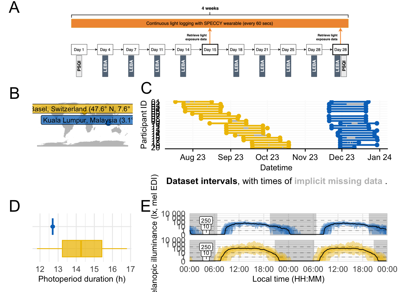
ggsave("figures/Figure_1.pdf", width = 17, height = 15, scale = 2, units = "cm")

# P5 + theme(plot.margin = margin(10,20,10,10),
#            axis.title = element_text(size = 12),
#         axis.text = element_text(size = 12))
# ggsave("figures/Average_Day.pdf", width = 8, height = 6, scale = 2, units = "cm")
6.5 Figure 2 Average day
data_1day <-
  data_combined %>%
  mutate(site = factor(site),
         dawn = hms::as_hms(dawn),
         dusk = hms::as_hms(dusk)) %>%
  filter(!marked_for_removal) %>%
  select(site, Id, Datetime, MEDI, dusk, dawn) %>%
  aggregate_Date(
    unit = "15 mins",
    mean_MEDI = mean(log10(MEDI), na.rm = TRUE),
    sd_MEDI = stats::sd(log10(MEDI), na.rm = TRUE),
    cv_MEDI = sd_MEDI/mean_MEDI,
    numeric.handler = \(x) median(x, na.rm = TRUE),
    lower95 = quantile(MEDI, 0.025, na.rm = TRUE),
    lower75 = quantile(MEDI, 0.125, na.rm = TRUE),
    lower50 = quantile(MEDI, 0.25, na.rm = TRUE),
    upper50 = quantile(MEDI, 0.75, na.rm = TRUE),
    upper75 = quantile(MEDI, 0.875, na.rm = TRUE),
    upper95 = quantile(MEDI, 0.975, na.rm = TRUE),
    dawn = mean(dawn, na.rm = TRUE),
    dusk = mean(dusk, na.rm = TRUE),
    date.handler = \(x) as_date("1970-01-01"),

  )

data_1day$dusk <-
  data_1day$dusk %>%
  hms::as_hms() %>%
  {paste("1970-01-01", .)} %>%
  parse_date_time(orders ="ymdHMS")
data_1day$dawn <-
  data_1day$dawn %>%
  hms::as_hms() %>%
  {paste("1970-01-01", .)} %>%
  parse_date_time(orders ="ymdHMS")

IS_data <-
  metrics$data[metrics$metric == "IS"][[1]] %>%
  mutate(Id = fct_relabel(Id, \(x) str_remove(x, "ID|MY0")),
         Id = factor(Id, levels = sprintf("%02d",1:20))) %>%
  mutate(site = site %>% fct_relabel(str_to_title))
photoperiod_1day <-
data_1day %>%
summarize(dawn = first((dawn)),
dusk = first((dusk)),
.groups = "drop")
hlinelabel <-
expand_grid(
site = c("Malaysia", "Switzerland"),
Id = sprintf("%02d", 1:20),
values = c(1, 10, 250)
) %>%
filter(!(site == "Malaysia" & Id == "06"))
facet_names <- c(Malaysia = "Kuala Lumpur, Malaysia",
Switzerland = "Basel, Switzerland")
singular_plot <-
data_1day %>%
ungroup() %>%
gg_doubleplot(
geom = "line", jco_color = FALSE, facetting = FALSE, col = "black",
alpha = 1,
y.axis.breaks = c(0, 1, 10, 1000, 100000)) +
geom_rect(data = photoperiod_1day,
aes(xmin = as_datetime("1970-01-01", tz = "UTC"),
xmax = dawn, ymin = -Inf, ymax = Inf), alpha = 0.25)+
geom_rect(data = photoperiod_1day,
aes(xmin = dusk, xmax = (dawn + ddays(1)), ymin = -Inf, ymax = Inf), alpha = 0.25)+
geom_rect(data = photoperiod_1day,
aes(xmin = dusk + ddays(1),
xmax = as_datetime("1970-01-03", tz = "UTC"),
ymin = -Inf, ymax = Inf), alpha = 0.25)+
facet_grid2(Id ~ site, switch = "y",
labeller = labeller(site = facet_names),
strip =
strip_themed(background_x = elem_list_rect(fill = pal_jco()(2)))) +
labs(fill = "Percentiles",
title = "Double plots of average days per participant ID and site",
subtitle =
"Median and percentiles of light exposure per 15 minutes (<span style='color:#ee0000AA;'>95%</span>, <span style='color:#ee0000CC;'>75%</span>, and <span style='color:#ee0000;'>50%</span> of data shown in ribbons). Grey backgrounds indicate (civil) nighttime. "
)+
theme(plot.subtitle = element_textbox_simple(padding = margin(b=10)))
singular_plot <-
singular_plot +
geom_ribbon(aes(ymin = lower95, ymax = upper95), fill = "red2", alpha = 0.25) +
geom_ribbon(aes(ymin = lower75, ymax = upper75), fill = "red2", alpha = 0.25) +
geom_ribbon(aes(ymin = lower50, ymax = upper50), fill = "red2", alpha = 0.25) +
geom_label(data = IS_data,
aes(x = as_datetime("1970-01-03", tz = "UTC") - dminutes(30),
y = 10^5, label = paste("IS =", value %>% round(2), "")),
hjust = 1,
vjust = 1,
alpha = 0.75
) +
theme(panel.spacing.x = unit(2.5, "lines")) +
ggplot2::scale_y_continuous(trans = "symlog",
breaks = c(0, 10^(0:5)), labels =
c("0", "", "10", "", "1 000", "", "100 000")
)
singular_plot$layers <-
c(singular_plot$layers[2:8], singular_plot$layers[1])
singular_plot <-
singular_plot +
map(c(1, 10, 250),
\(x) geom_hline(aes(yintercept = !!x), linetype = 2, , alpha = 0.25)
) +
geom_label(data = hlinelabel, aes(y = values, label = values,
x = as_datetime("1970-01-01 04:00:00",
tz = "UTC")),
size = 2.5) +
labs(x = "Local time (HH:MM)", y = "Melanopic illuminance (lx, mel EDI)")
singular_plot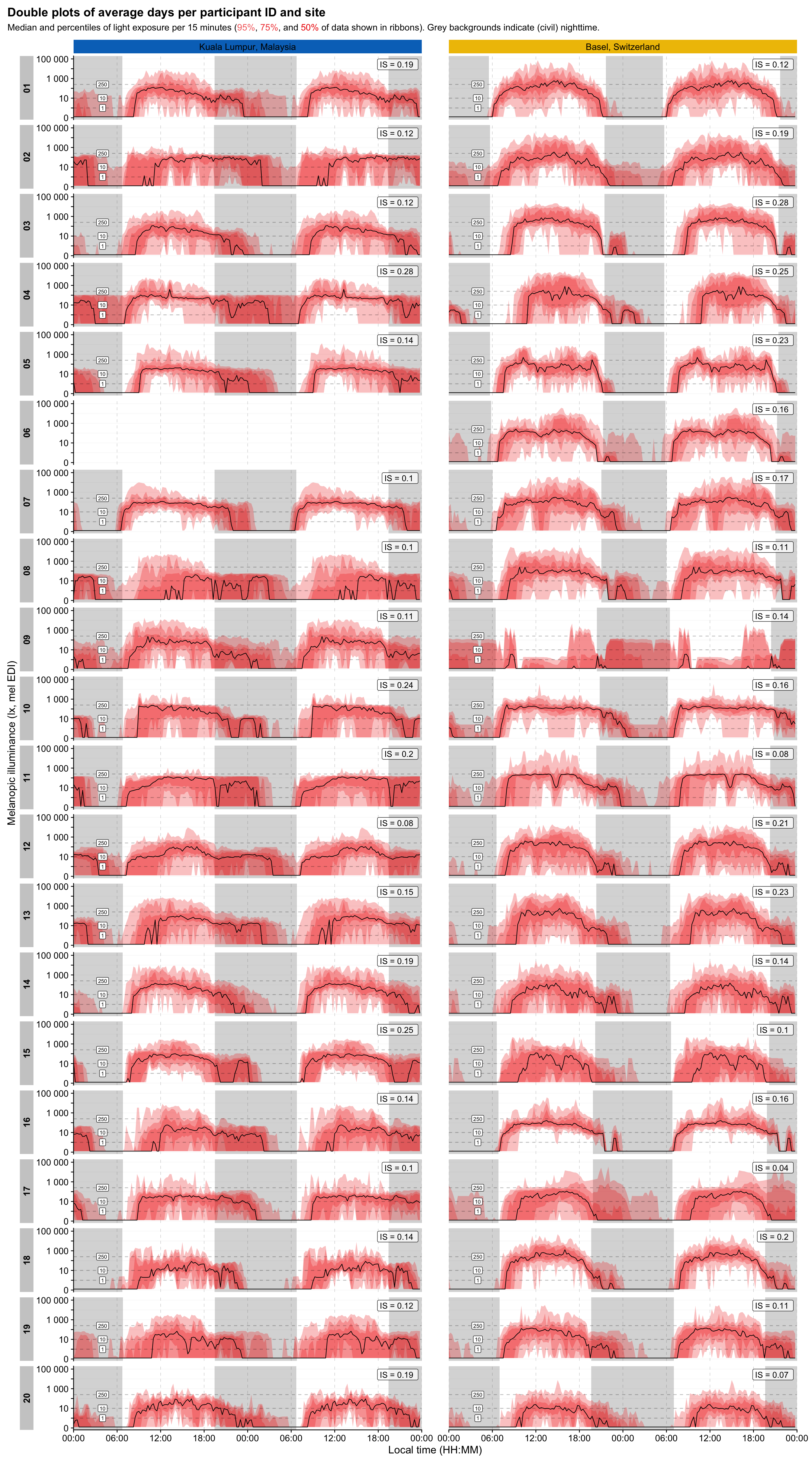
ggsave("figures/Figure_2.pdf", singular_plot,
       width = 17, height = 25, units = "cm",scale = 2)
6.6 Figure 3 Chronotype influence on light exposure timing
This figure was added as part of revision 1 and can be found below under section Section 7.4.
6.7 Figure 4 Daily patterns
light_pattern <-
plot_smooth(
  Pattern_model,
  view = "Time",
  plot_all = "site",
  rug = F,
  n.grid = 90,
  col = pal_jco()(2),
  rm.ranef = "s(Id)",
  sim.ci = TRUE,
  )
Summary:
* site : factor; set to the value(s): malaysia, switzerland.
* Time : numeric predictor; with 200 values ranging from 0.000000 to 23.983333.
* Id : factor; set to the value(s): MY012.
* NOTE : The following random effects columns are canceled: s(Time):sitemalaysia,s(Time):siteswitzerland,s(Id):sitemalaysia,s(Id):siteswitzerland
* Simultaneous 95%-CI used :
Critical value: 2.355
Proportion posterior simulations in pointwise CI: 0.87 (10000 samples)
Proportion posterior simulations in simultaneous CI: 0.95 (10000 samples)

light_pattern_diff <-
plot_diff(Pattern_model,
          view = "Time",
          rm.ranef = "s(Id)",
          comp = list(site = c("malaysia", "switzerland")),
          sim.ci = TRUE,
          n.grid = 10000)
Summary:
* Time : numeric predictor; with 10000 values ranging from 0.000000 to 23.983333.
* Id : factor; set to the value(s): MY012.
* NOTE : The following random effects columns are canceled: s(Time):sitemalaysia,s(Time):siteswitzerland,s(Id):sitemalaysia,s(Id):siteswitzerland
* Simultaneous 95%-CI used :
Critical value: 2.087
Proportion posterior simulations in pointwise CI: 1 (10000 samples)
Proportion posterior simulations in simultaneous CI: 1 (10000 samples)
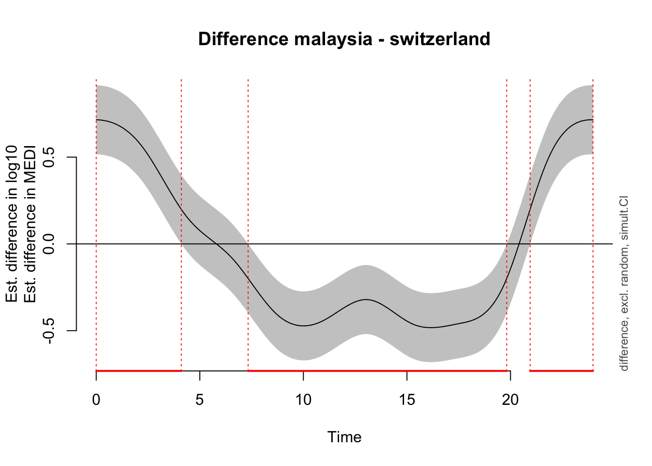
Time window(s) of significant difference(s):
    0.000000 - 4.106357
    7.332438 - 19.817012
    20.946740 - 23.983333
light_pattern_individuals <-
plot_smooth(
Pattern_modelm1,
view = "Time",
plot_all = "Id",
rm.ranef = FALSE,
se = 0,
rug = F,
n.grid = 90,
col = c(rep(colors_pattern[1], 19),rep(colors_pattern[2], 20)),
sim.ci = TRUE
)Summary:
* Time : numeric predictor; with 200 values ranging from 0.000000 to 23.983333.
* Id : factor with 39 values; set to the value(s): ID01, ID02, ID03, ID04, ID05, ID06, ID07, ID08, ID09, ID10, ...
* site : factor; set to the value(s): switzerland.
* Simultaneous 95%-CI used :
Critical value: 3.939
Proportion posterior simulations in pointwise CI: 1 (10000 samples)
Proportion posterior simulations in simultaneous CI: 0.95 (10000 samples)
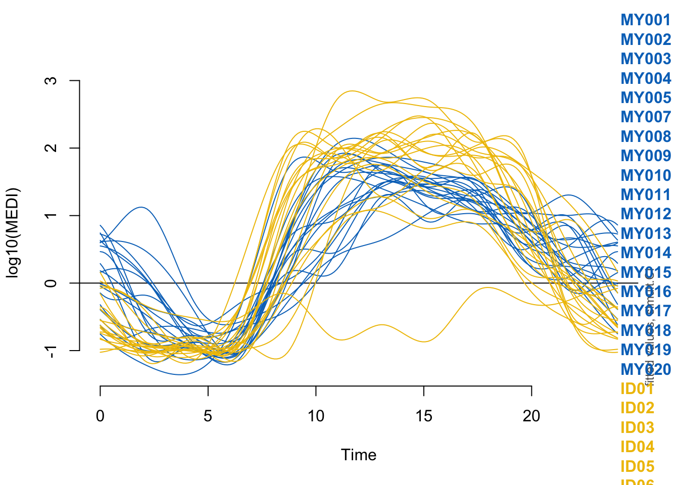
time_labels <- c("00:00", "06:00", "12:00", "18:00", "24:00")

P1 <-
light_pattern$fv %>%
  mutate(site = str_to_title(site)) %>%
  ggplot(aes(x = Time*60*60, y = fit, col = site)) +
  geom_ribbon(aes(ymin = ll, ymax = ul, fill = site), alpha = 0.25, col = NA)+
  geom_line() +
  theme_minimal() +
  scale_color_jco()+
  scale_fill_jco()+
  labs(y = "Model fit with 95% CI, log10(mel EDI, lx)", x = "Local Time (HH:MM)",
       color = "Site", fill = "Site") +
  scale_x_time(limits = c(0, 24*60*60), expand = c(0,0),
               breaks = c(0, 6, 12, 18, 24)*60*60, labels = time_labels
               )

label_sig <- "Credible non-\nzero difference"

P2 <-
light_pattern_diff %>%
  mutate(significant = (est-sim.CI < 0) & (0 < est + sim.CI)) %>%
  ggplot(aes(x = Time*60*60, y = est, group = consecutive_id(significant) )) +
  geom_ribbon(aes(ymin = est-sim.CI, ymax = est+sim.CI, fill = !significant),
              alpha = 0.25, col = NA)+
  geom_line(aes(col = !significant)) +
  geom_hline(aes(yintercept = 0)) +
  theme_minimal() +
  labs(y = "Fitted difference smooth with 95% CI", x = NULL,
       col = label_sig, fill = label_sig) +
  scale_x_time(limits = c(0, 24*60*60), expand = c(0,0),
               breaks = c(0, 6, 12, 18, 24)*60*60, labels = time_labels)

P3 <-
light_pattern_individuals$fv %>%
  mutate(site = str_detect(Id, "MY"),
         site = if_else(site, "Malaysia", "Switzerland")) %>%
  ggplot(aes(x = Time*60*60, y = fit, col = site, group = Id)) +
  # geom_ribbon(aes(ymin = ll, ymax = ul, fill = site), alpha = 0.25, col = NA)+
  geom_line() +
  theme_minimal() +
  scale_color_jco()+
  scale_fill_jco()+
  labs(y = "Model fit, log10(mel EDI, lx)", x = NULL, col = "Site", fill = "Site") +
  scale_x_time(limits = c(0, 24*60*60), expand = c(0,0),
               breaks = c(0, 6, 12, 18, 24)*60*60, labels = time_labels) +
  theme(legend.position = "none")

(P3 + P1 + P2) +
  plot_annotation(tag_levels = "A") +
  plot_layout(guides = "collect")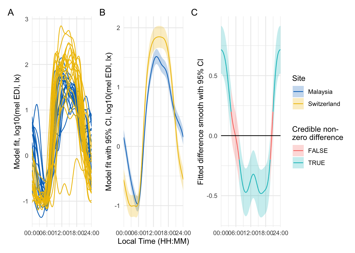
ggsave("figures/Figure_4.pdf",
       width = 17, height = 7, units = "cm", scale = 1.6)
6.8 Figure 5 Correlation Matrix
#visualization
(corr_plot_malaysia + theme(legend.position = "none")) +
  (corr_plot_switzerland) +
  # plot_layout(guides = "collect")+
  theme(legend.position = "bottom",
        legend.justification = c(1,1))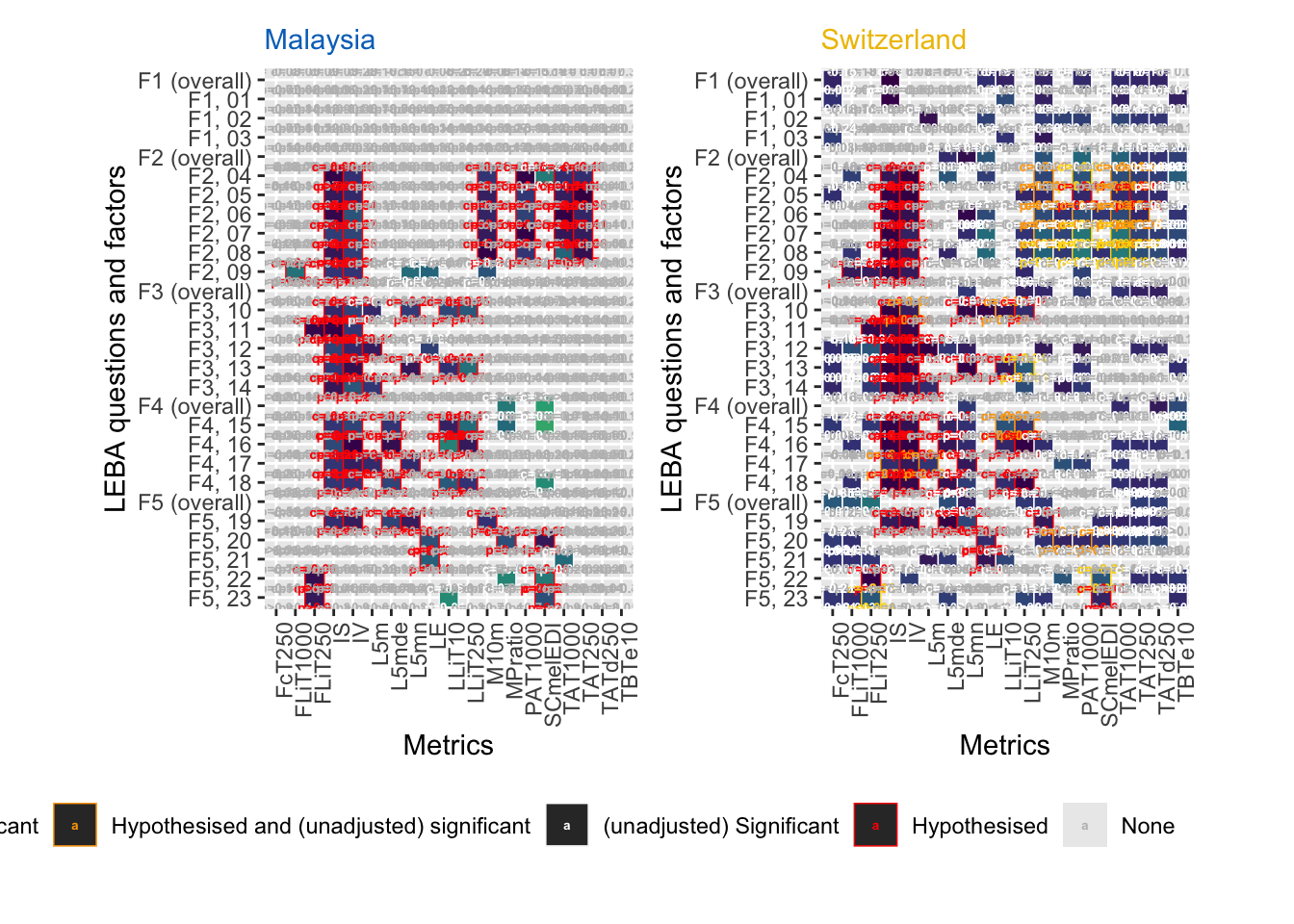
ggsave("figures/Figure_5.pdf",
       width = 25, height = 17, units = "cm", scale = 1.6)
6.9 S1 Missing time: Bootstrap results
bootstrap_0 <-
bootstrap_comparison %>%
  filter(threshold == 1) %>%
  mutate(across(contains("bs"), \(x) mean),
         threshold = 0)

bootstrap_0 %>%
  rbind(bootstrap_comparison) %>%
  ggplot(aes(x = threshold)) +
    geom_ribbon(aes(ymin = (mean - 2*se), ymax = (mean + 2*se)),
                fill = "steelblue", alpha = 0.4) +
  geom_hline(data = subset_metrics, aes(yintercept=mean), color = "steelblue") +
  geom_errorbar(
    aes(ymin = lower_bs1, ymax = upper_bs1), linewidth = 0.5, width = 0) +
  geom_errorbar(aes(ymin = lower_bs2, ymax = upper_bs2),
                linewidth = 0.25, width = 0) +
  geom_point(aes(y=mean_bs,
                 col = ((mean - 2*se) <= lower_bs3 & upper_bs3 <= (mean + 2*se)))) +
  facet_wrap(Id~metric, scales = "free") +
  theme_minimal() +
  labs(x = "Hours missing from the day", y = "Metric value", col = "Within Range") +
  theme(legend.position = "bottom") +
  coord_cartesian(xlim = c(0, 21), expand = FALSE, clip = FALSE) +
  geom_text(
    data =
      bootstrap_comparison %>%
      filter((mean - 2*se) <= lower_bs3 & upper_bs3 <= (mean + 2*se)) %>%
      group_by(metric, Id) %>%
      filter(threshold == max(threshold)),
    aes(label = threshold, x = threshold, y = mean_bs),
    size = 2.5,
  )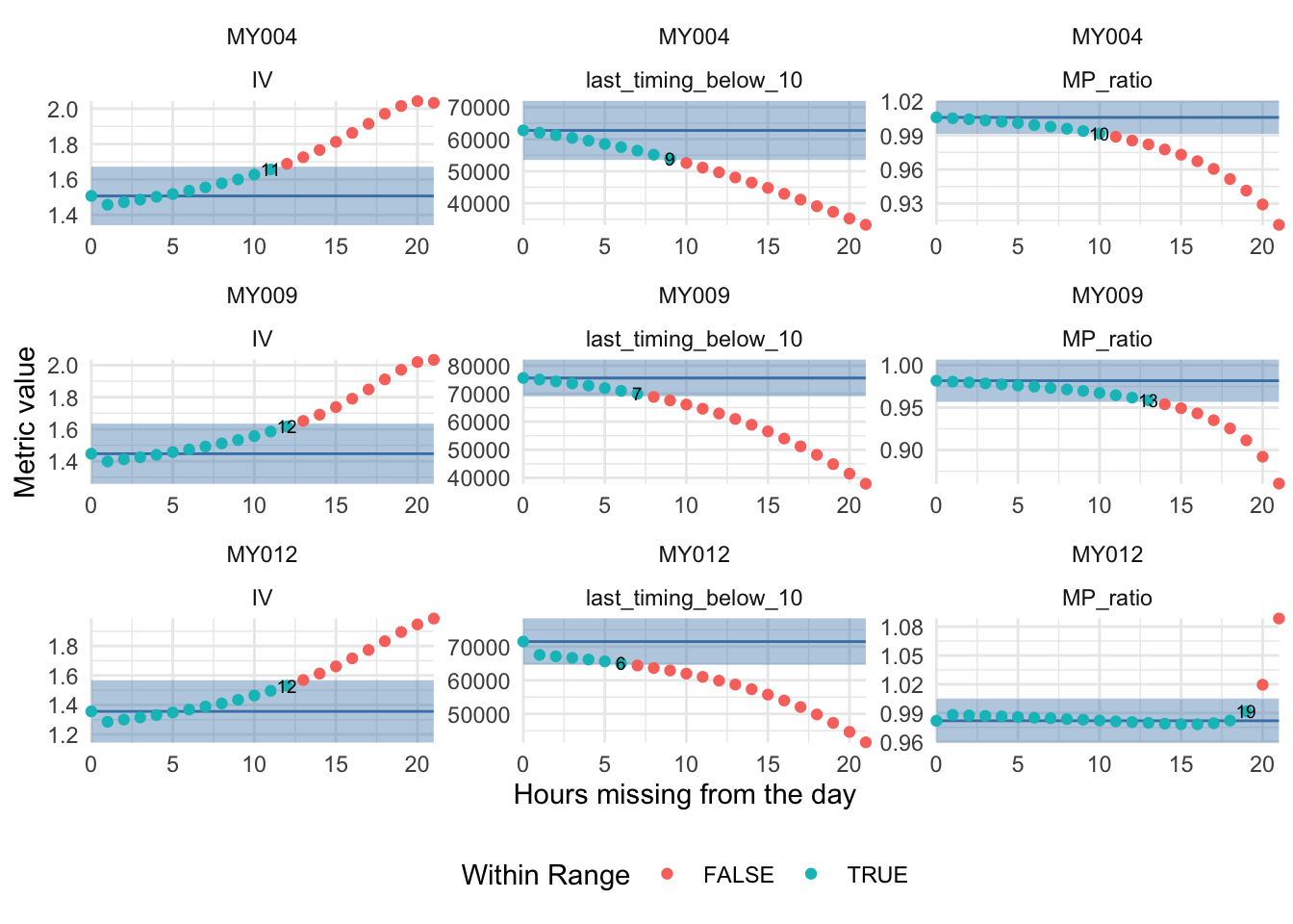
ggsave("figures/Figure_S1.pdf",
       width = 10, height = 7, units = "cm", scale = 2)
7 Revision 1
The following analysis were added during a revision of the manuscript following reviewer feedback
#import data on sex and age
demographic_data <- read_excel("data/LEBA_Participants_Age_Sex.xlsx")
demographic_data$site <- c(rep(c("switzerland"), 20), rep("malaysia", 19))
demographic_data <- demographic_data |> mutate(age_c = scale(age, scale = FALSE),
                                               age_m = mean(age))
demographic_data <- demographic_data |>
  mutate(age_cs = scale(age, scale = FALSE),
         age_ms = mean(age), .by = site)

#collect the light exposure data
le_data <- metrics %>% filter(metric == "MEDI") %>% pull(data) %>% .[[1]]
#add sex and age data
le_data <-
  le_data |>
  left_join(demographic_data, by = join_by(site, Id)) |>
  mutate(Id = factor(Id), site = factor(site))
7.1 Sex differences in light exposure
We explore sex differences in the light exposure pattern of the sites
le_data$site_sex <- interaction(le_data$site, le_data$sex, drop = TRUE)   # 4-level factor
le_data$sex <- factor(le_data$sex)

form1 <- log10(MEDI) ~
          site * sex +                        # parametric means
          s(Time, by = site_sex, bs = "cc", k = 12) +      # four separate curves
          s(Id, bs = "re")             # id-level random intercepts

form0 <- log10(MEDI) ~
          site +                        # parametric means
          s(Time, by = site, bs = "cc", k = 12) +      # four separate curves
          s(Id, bs = "re")             # id-level random intercepts

#setting the ends for the cyclic smooth
knots_day <- list(Time = c(0, 24))

#Model generation
sex_model <-
  bam(formula = form1,
      data = le_data,
      knots = knots_day,
      samfrac = 0.1,
      discrete = FALSE,
      nthreads = 4,
      control = list(nthreads = 4)
      )

sex_model0 <-
  bam(formula = form0,
      data = le_data,
      knots = knots_day,
      samfrac = 0.1,
      discrete = FALSE,
      nthreads = 4,
      control = list(nthreads = 4)
      )

#Model performance
AICs <-
AIC(sex_model0, sex_model)
AICs
df AIC
sex_model0 59.97069 4516271
sex_model 79.90582 4506167sex_model_sum <-
summary(sex_model)
sex_model_sum
Family: gaussian
Link function: identity

Formula:
log10(MEDI) ~ site * sex + s(Time, by = site_sex, bs = "cc",
    k = 12) + s(Id, bs = "re")

Parametric coefficients:
                     Estimate Std. Error t value Pr(>|t|)
(Intercept)           0.37533    0.08867   4.233 2.31e-05 ***
siteswitzerland       0.16833    0.11674   1.442   0.1493
sexM                  0.18664    0.13665   1.366   0.1720
siteswitzerland:sexM -0.37610    0.20430  -1.841   0.0656 .
---
Signif. codes:  0 '***' 0.001 '**' 0.01 '*' 0.05 '.' 0.1 ' ' 1

Approximate significance of smooth terms:
                                 edf Ref.df     F p-value
s(Time):site_sexmalaysia.F     9.976     10 20933  <2e-16 ***
s(Time):site_sexswitzerland.F  9.993     10 67145  <2e-16 ***
s(Time):site_sexmalaysia.M     9.981     10 16893  <2e-16 ***
s(Time):site_sexswitzerland.M  9.949     10 12652  <2e-16 ***
s(Id)                         34.985     35  2108  <2e-16 ***
---
Signif. codes:  0 '***' 0.001 '**' 0.01 '*' 0.05 '.' 0.1 ' ' 1

R-sq.(adj) =  0.458   Deviance explained = 45.8%
fREML = 2.2534e+06 Scale est. = 1.2561 n = 1469740gam.check(sex_model)
Method: fREML   Optimizer: perf newton
full convergence after 11 iterations.
Gradient range [-0.01322927,0.0130407]
(score 2253354 & scale 1.256123).
Hessian positive definite, eigenvalue range [4.951383,734868].
Model rank =  83 / 83

Basis dimension (k) checking results. Low p-value (k-index<1) may
indicate that k is too low, especially if edf is close to k'.

                                 k'   edf k-index p-value
s(Time):site_sexmalaysia.F    10.00  9.98    0.99    0.21
s(Time):site_sexswitzerland.F 10.00  9.99    0.99    0.24
s(Time):site_sexmalaysia.M    10.00  9.98    0.99    0.30
s(Time):site_sexswitzerland.M 10.00  9.95    0.99    0.28
s(Id)                         39.00 34.98      NA      NA
# plot(Pattern_model)
draw(sex_model)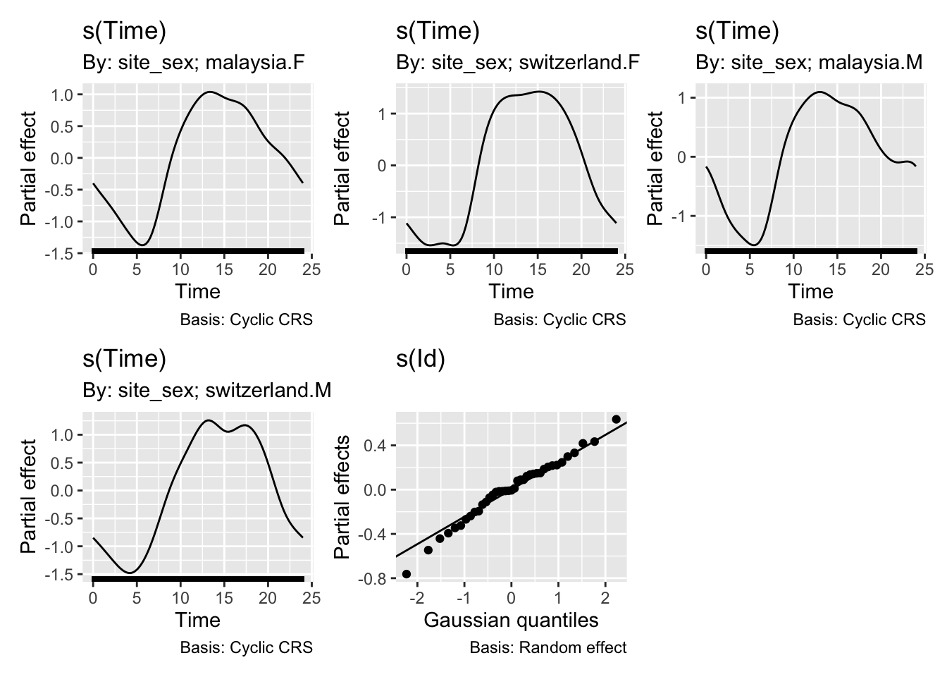
sex_plot_o <-
plot_smooth(
  sex_model,
  view = "Time",
  plot_all = c("site_sex", "sex", "site"),
  rug = F,
  n.grid = 90,
  col = c(pal_jco()(2), pal_jco()(2) |> alpha(0.5)),
  rm.ranef = "s(Id)",
  sim.ci = TRUE
  )
Summary:
* site : factor; set to the value(s): malaysia, switzerland.
* sex : factor; set to the value(s): F, M.
* Time : numeric predictor; with 200 values ranging from 0.000000 to 23.983333.
* site_sex : factor; set to the value(s): malaysia.F, malaysia.M, switzerland.F, switzerland.M.
* Id : factor; set to the value(s): ID07. (Might be canceled as random effect, check below.)
* NOTE : The following random effects columns are canceled: s(Time):site_sexmalaysia.F,s(Time):site_sexswitzerland.F,s(Time):site_sexmalaysia.M,s(Time):site_sexswitzerland.M,s(Id)
* Simultaneous 95%-CI used :
Critical value: 2.664
Proportion posterior simulations in pointwise CI: 0.72 (10000 samples)
Proportion posterior simulations in simultaneous CI: 0.95 (10000 samples)
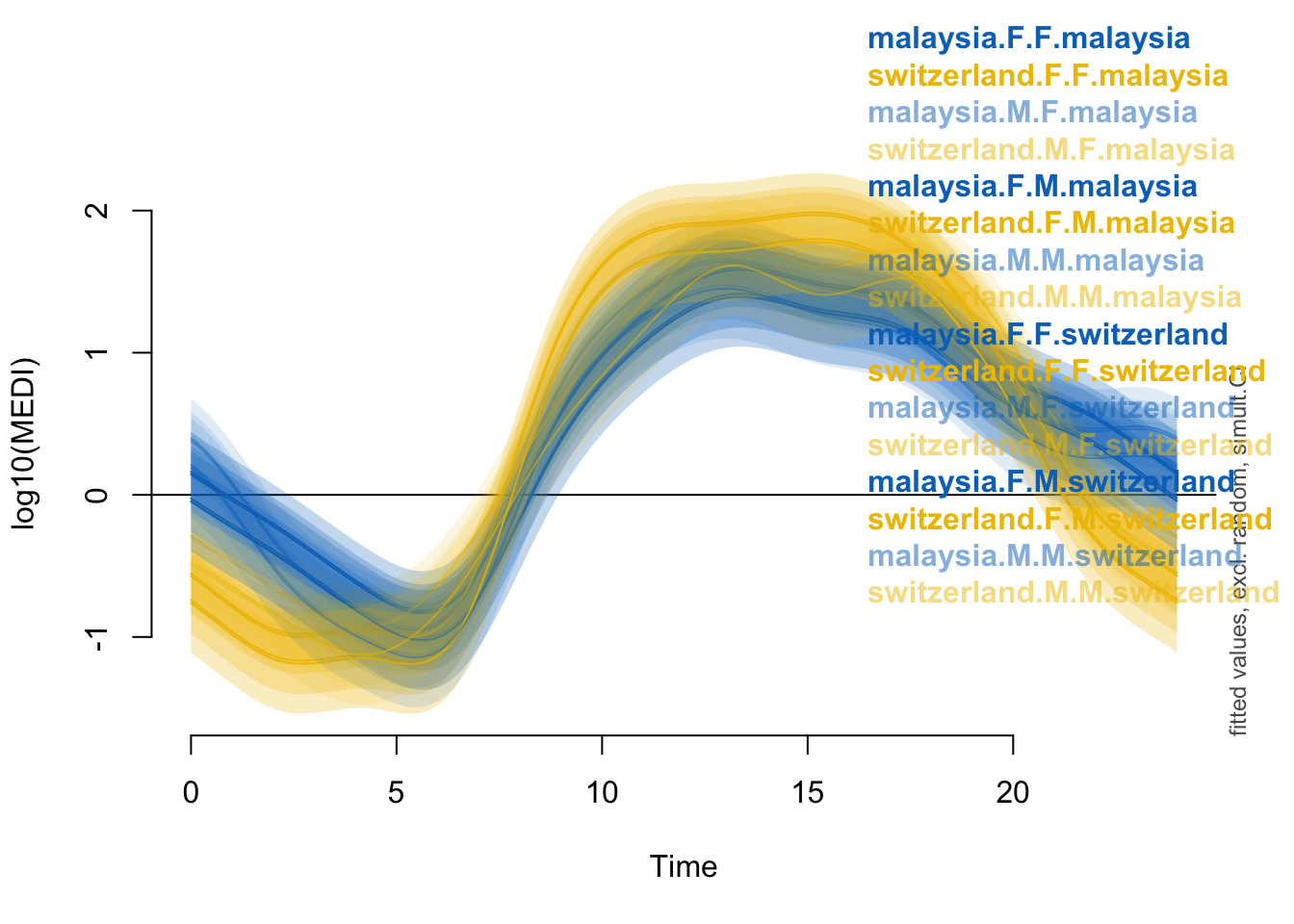
sex_plot_d1 <-
plot_diff(sex_model,
          view = "Time",
          rm.ranef = "s(Id)",
          cond = list(site = "switzerland"),
          comp = list(sex = c("F", "M"), site_sex = c("switzerland.F", "switzerland.M")),
          sim.ci = TRUE)
Summary:
* site : factor; set to the value(s): switzerland.
* Time : numeric predictor; with 200 values ranging from 0.000000 to 23.983333.
* Id : factor; set to the value(s): ID07. (Might be canceled as random effect, check below.)
* NOTE : The following random effects columns are canceled: s(Time):site_sexmalaysia.F,s(Time):site_sexswitzerland.F,s(Time):site_sexmalaysia.M,s(Time):site_sexswitzerland.M,s(Id)
* Simultaneous 95%-CI used :
Critical value: 2.067
Proportion posterior simulations in pointwise CI: 1 (10000 samples)
Proportion posterior simulations in simultaneous CI: 1 (10000 samples)
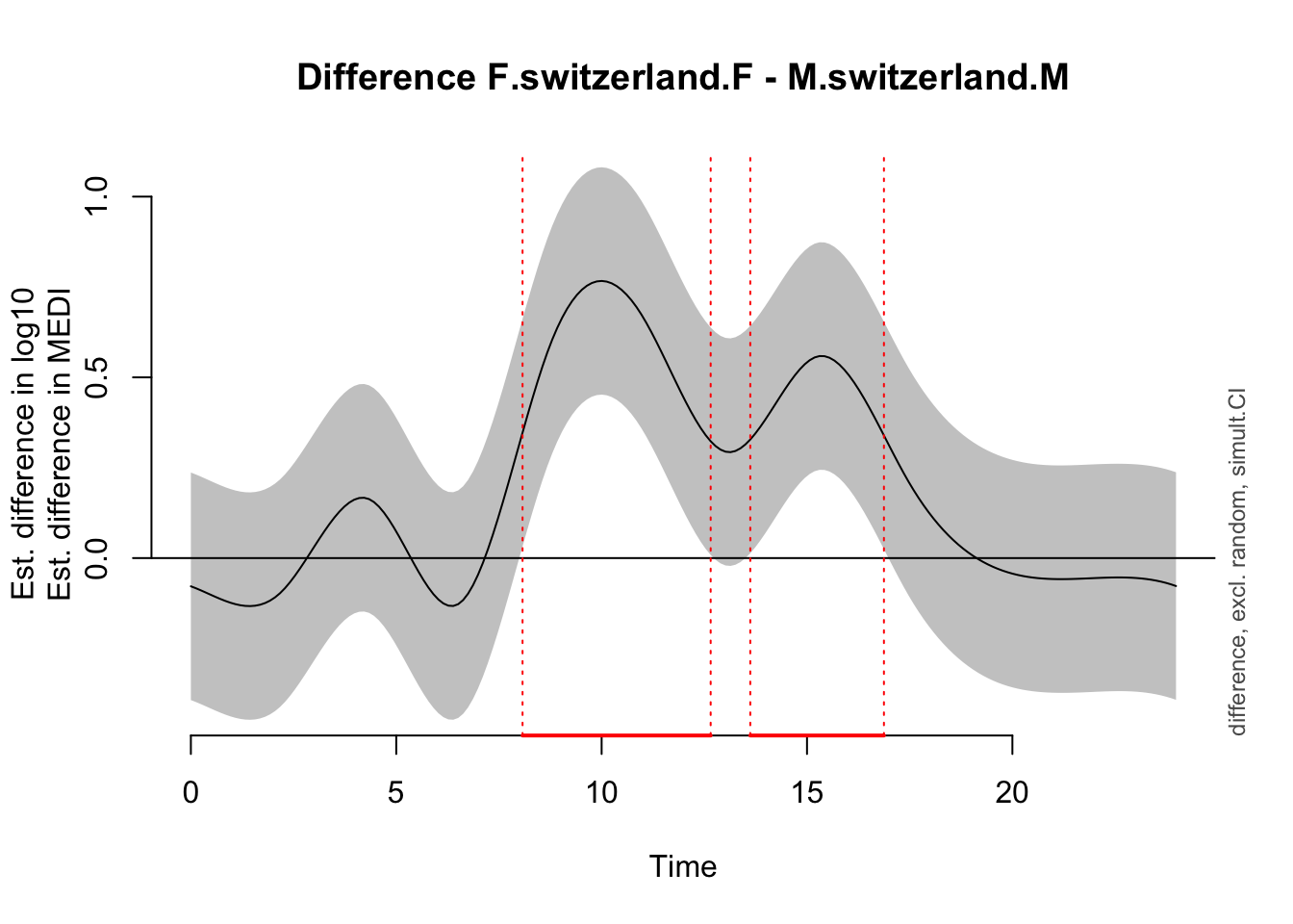
Time window(s) of significant difference(s):
    8.074791 - 12.654523
    13.618677 - 16.872697
sex_plot_d2 <-
plot_diff(sex_model,
view = "Time",
rm.ranef = "s(Id)",
cond = list(site = "malaysia"),
comp = list(sex = c("F", "M"), site_sex = c("malaysia.F", "malaysia.M")),
sim.ci = TRUE)Summary:
* site : factor; set to the value(s): malaysia.
* Time : numeric predictor; with 200 values ranging from 0.000000 to 23.983333.
* Id : factor; set to the value(s): ID07. (Might be canceled as random effect, check below.)
* NOTE : The following random effects columns are canceled: s(Time):site_sexmalaysia.F,s(Time):site_sexswitzerland.F,s(Time):site_sexmalaysia.M,s(Time):site_sexswitzerland.M,s(Id)
* Simultaneous 95%-CI used :
Critical value: 2.089
Proportion posterior simulations in pointwise CI: 1 (10000 samples)
Proportion posterior simulations in simultaneous CI: 1 (10000 samples)
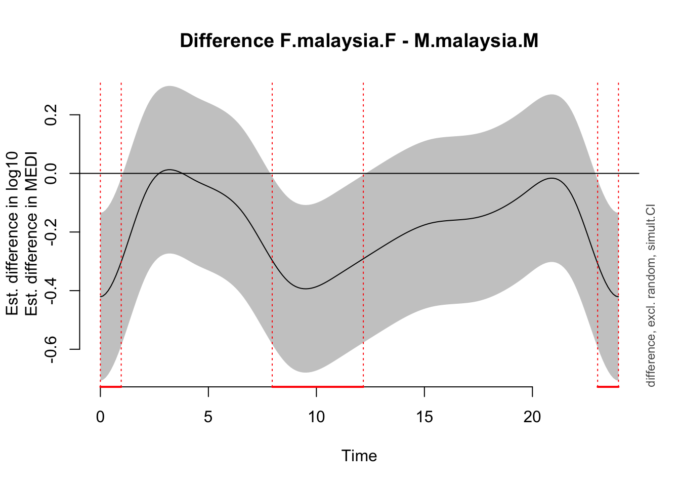
Time window(s) of significant difference(s):
    0.000000 - 0.964154
    7.954271 - 12.172446
    23.019179 - 23.983333
Psex1 <-
sex_plot_o$fv %>%
filter(str_detect(site_sex, c(as.character(site)))) |>
filter(str_detect(site_sex, c(as.character(sex)))) |>
mutate(site = str_to_title(site),) %>%
ggplot(aes(x = Time*60*60, y = fit, col = site_sex, lty = sex)) +
geom_ribbon(aes(ymin = ll, ymax = ul, fill = site_sex), alpha = 0.25, col = NA)+
geom_line() +
theme_minimal() +
scale_color_manual(values = c("#0073C2FF", "#EFC000FF", "#0073C2FF", "#EFC000FF")) +
scale_fill_manual(values = c("#0073C280", "#EFC00080", "#0073C240", "#EFC00040")) +
scale_linetype_manual(values = c(1, 2)) +
# scale_color_jco()+
# scale_fill_jco()+
labs(y = "Model fit with 95% CI, log10(mel EDI, lx)", x = "Local Time (HH:MM)",
linetype = "Sex") +
guides(fill = "none", color = "none") +
scale_x_time(limits = c(0, 24*60*60), expand = c(0,0),
breaks = c(0, 6, 12, 18, 24)*60*60, labels = time_labels
) +
facet_wrap(~site) +
theme(panel.spacing = unit(1.75, "lines"))
Psex2 <-
sex_plot_d1 %>%
mutate(significant = (est-sim.CI < 0) & (0 < est + sim.CI),
site = "Switzerland (F - M)") %>%
ggplot(aes(x = Time*60*60, y = est, group = consecutive_id(significant) )) +
geom_ribbon(aes(ymin = est-sim.CI, ymax = est+sim.CI, fill = !significant),
alpha = 0.25, col = NA)+
geom_line(aes(col = !significant)) +
geom_hline(aes(yintercept = 0)) +
theme_minimal() +
facet_wrap(~site) +
labs(y = "Fitted difference smooth with 95% CI", x = NULL,
col = label_sig, fill = label_sig) +
scale_x_time(limits = c(0, 24*60*60), expand = c(0,0),
breaks = c(0, 6, 12, 18, 24)*60*60, labels = time_labels)
Psex3 <-
sex_plot_d2 %>%
mutate(significant = (est-sim.CI < 0) & (0 < est + sim.CI),
site = "Malaysia (F - M)") %>%
ggplot(aes(x = Time*60*60, y = est, group = consecutive_id(significant) )) +
geom_ribbon(aes(ymin = est-sim.CI, ymax = est+sim.CI, fill = !significant),
alpha = 0.25, col = NA)+
geom_line(aes(col = !significant)) +
geom_hline(aes(yintercept = 0)) +
theme_minimal() +
labs(y = "Fitted difference smooth with 95% CI", x = NULL,
col = label_sig, fill = label_sig) +
facet_wrap(~site) +
scale_x_time(limits = c(0, 24*60*60), expand = c(0,0),
breaks = c(0, 6, 12, 18, 24)*60*60, labels = time_labels)
(Psex1 + Psex3 + Psex2) +
plot_annotation(tag_levels = "A") +
plot_layout(guides = "collect",widths = c(2,1,1))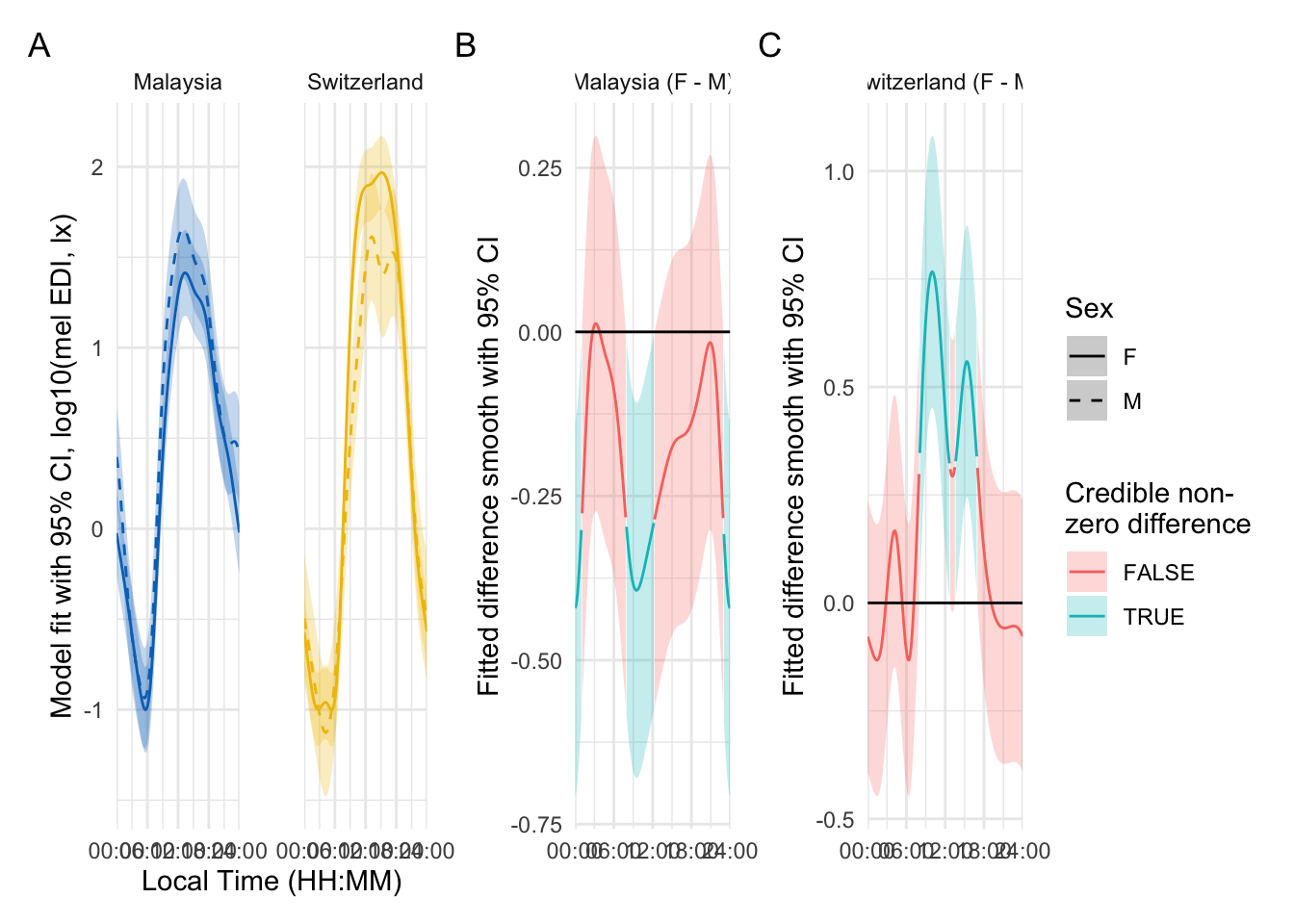
ggsave("figures/Figure_S2.pdf",
       width = 17, height = 7, units = "cm", scale = 1.6)
There is strong evidence for a site specific effect of sex. While there is no difference in overall melanopic EDI, the patterns of exposure differ. Specifically, females in Malaysia are less exposed to light in the hours before noon and around midnight, compared to males. In Switzerland, females are exposed to more light before noon, compared to males, and are also more likely to have a higher exposure in the afternoon. The effect size is a reduction of about 60% for women in Malaysia in the specified times of day, and about a 5-fold increase for women in Switzerland before noon, and about 2- to 3-fold in the afternoon.
TAT1000 <- metrics |> filter(metric == "TAT1000")
TAT1000 <-
TAT1000 |>
  mutate(data = data |> map(
    \(x) x |>
      left_join(demographic_data, by = join_by(site, Id)) |>
      mutate(Id = factor(Id), site = factor(site)))
  )

formula_Hsex <- value ~ site*sex + (1|site:Id)
formula_H0sex <- value ~ site + (1|site:Id)

map <- purrr::map

inference_Hsex <-
  TAT1000 %>%
  # mutate(data =
  #          data %>%
  #          purrr::map(\(x) x %>% mutate(value_dc =
  #                                  (value/photoperiod_duration) %>% round()))
  #        )
  inference_summary(formula_Hsex, formula_H0sex, p_adjustment = 1,
                    family = poisson())
m_sex1 <- glmer(formula_Hsex, data = TAT1000$data[[1]], family = poisson())
m_sex0 <- glmer(formula_H0sex, data = TAT1000$data[[1]], family = poisson())

summary(m_sex1)
Generalized linear mixed model fit by maximum likelihood (Laplace
Approximation) [glmerMod]
Family: poisson ( log )
Formula: value ~ site * sex + (1 | site:Id)
Data: TAT1000$data[[1]]
AIC BIC logLik -2*log(L) df.resid
3724896 3724921 -1862443 3724886 1018
Scaled residuals:
Min 1Q Median 3Q Max
-96.36 -43.08 -15.91 25.25 374.11
Random effects:
Groups Name Variance Std.Dev.
site:Id (Intercept) 0.4124 0.6422
Number of obs: 1023, groups: site:Id, 39
Fixed effects:
Estimate Std. Error z value Pr(>|z|)
(Intercept) 7.76346 0.18716 41.480 < 2e-16 ***
siteswitzerland 0.85641 0.24617 3.479 0.000503 ***
sexM -0.07439 0.29177 -0.255 0.798743
siteswitzerland:sexM -0.35411 0.43955 -0.806 0.420462
---
Signif. codes: 0 '***' 0.001 '**' 0.01 '*' 0.05 '.' 0.1 ' ' 1
Correlation of Fixed Effects:
(Intr) stswtz sexM
sitswtzrlnd -0.747
sexM -0.634 0.473
stswtzrln:M 0.412 -0.555 -0.658summary(m_sex0)Generalized linear mixed model fit by maximum likelihood (Laplace
Approximation) [glmerMod]
Family: poisson ( log )
Formula: value ~ site + (1 | site:Id)
Data: TAT1000$data[[1]]
AIC BIC logLik -2*log(L) df.resid
3724894 3724908 -1862444 3724888 1020
Scaled residuals:
Min 1Q Median 3Q Max
-96.36 -43.08 -15.91 25.25 374.11
Random effects:
Groups Name Variance Std.Dev.
site:Id (Intercept) 0.4307 0.6563
Number of obs: 1023, groups: site:Id, 39
Fixed effects:
Estimate Std. Error z value Pr(>|z|)
(Intercept) 7.7321 0.1499 51.588 < 2e-16 ***
siteswitzerland 0.7806 0.2091 3.734 0.000189 ***
---
Signif. codes: 0 '***' 0.001 '**' 0.01 '*' 0.05 '.' 0.1 ' ' 1
Correlation of Fixed Effects:
(Intr)
sitswtzrlnd -0.715anova(m_sex1, m_sex0)Data: TAT1000$data[[1]]
Models:
m_sex0: value ~ site + (1 | site:Id)
m_sex1: value ~ site * sex + (1 | site:Id)
npar AIC BIC logLik -2*log(L) Chisq Df Pr(>Chisq)
m_sex0 3 3724894 3724908 -1862444 3724888
m_sex1 5 3724896 3724921 -1862443 3724886 1.6942 2 0.4287There is no significant difference between the time spent above 1000 lx between men or women in either of the sites.
7.2 Age differences in light exposure
We explore age differences in the sites, starting with some basic comparisons.
sex_lab <- primitive_bracket(
  key  = key_range_manual(          # <− positions + labels
    start = c(-7,0.1),

    end = c(-0.1,7),# -6  and  +6  on the x-axis
    name     = c("Males", "Females")
  ),
  position = "bottom"         # draw it at the bottom of the panel
)

demographic_data |>
  mutate(
         age_group =
           cut(age,
               breaks = seq(15,55,5),
               labels = c("18-20", "21-25", "26-30", "31-35", "36-40", "41-45", "46-50", "51-55"),
               right = FALSE),
         site = str_to_title(site)
         )|>
  group_by(site, sex, age_group) |>
  summarize(n = n(), .groups = "drop") |>
  mutate(n = ifelse(sex == "M", -n, n)) |>
  ggplot(aes(x= age_group, y = n, alpha = sex, fill = site)) +
  geom_col() +
  geom_hline(yintercept = 0) +
  facet_wrap(~site) +
  scale_y_continuous(breaks = seq(-6,6, by = 2),
                     labels = c(6, 4, 2, 0, 2, 4, 6)) +
  scale_fill_manual(values = pal_jco()(2)) +
  scale_alpha_manual(values = c(1, 1))+
  guides(fill = "none", alpha = "none",
         x = guide_axis_stack(
           "axis", sex_lab
         )) +
  theme_minimal() +
  coord_flip(ylim = c(-7, 7)) +
  labs(x = "Age (yrs)", y = "n", fill = "Site")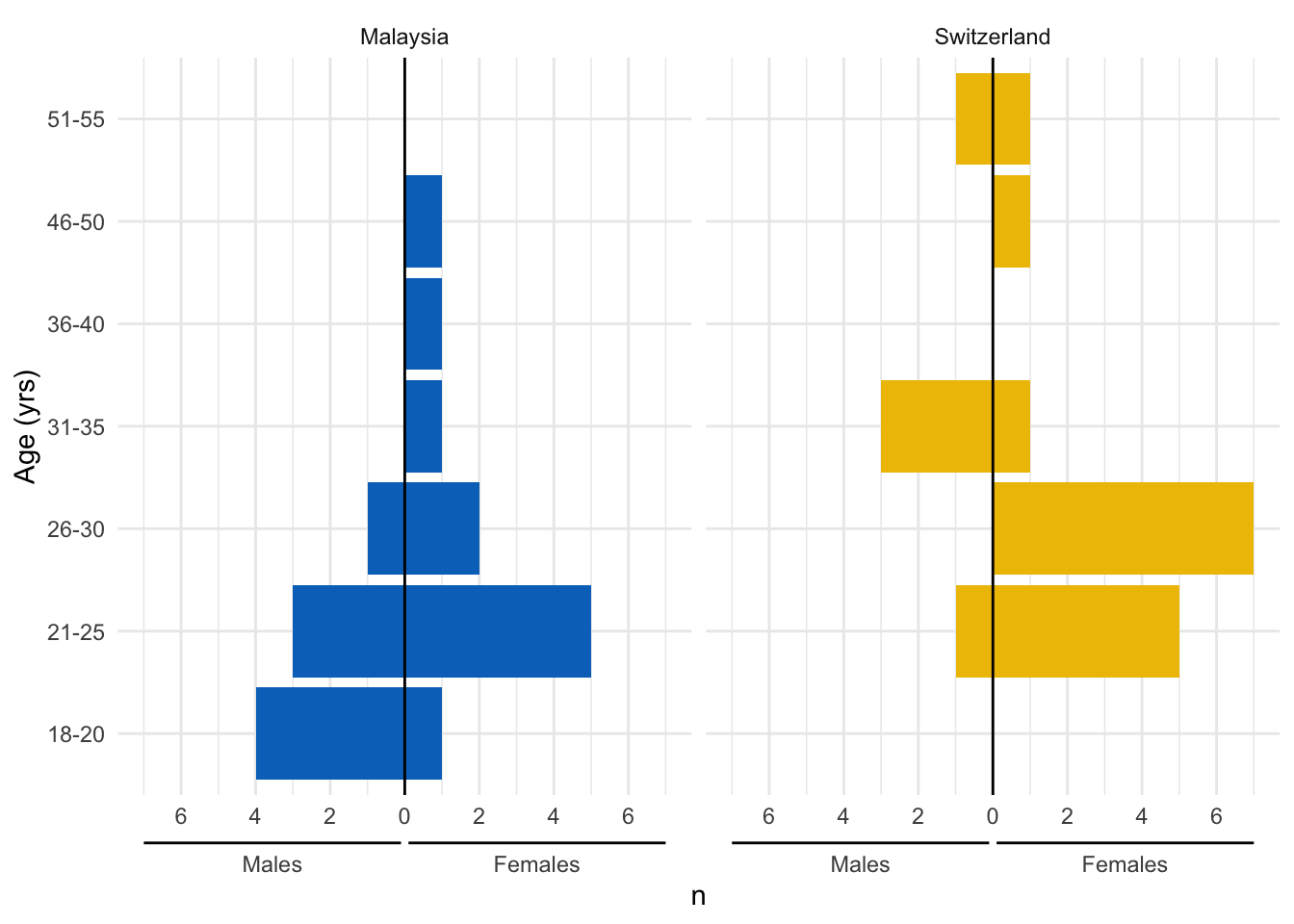
ggsave("figures/Figure_S3.pdf",
       width = 10, height = 6, units = "cm", scale = 1.6)

model_age <- lm(age ~ site*sex, data = demographic_data)
model_age2 <- lm(age ~ site +sex, data = demographic_data)
model_age3 <- lm(age ~ site, data = demographic_data)
model_age |> summary()
Call:
lm(formula = age ~ site * sex, data = demographic_data)

Residuals:
     Min       1Q   Median       3Q      Max
-12.0000  -4.8000  -2.0000   0.9091  24.2000

Coefficients:
                     Estimate Std. Error t value Pr(>|t|)
(Intercept)            26.182      2.528  10.358 3.35e-12 ***
siteswitzerland         2.618      3.328   0.787   0.4367
sexM                   -5.182      3.896  -1.330   0.1921
siteswitzerland:sexM   11.382      5.824   1.954   0.0587 .
---
Signif. codes:  0 '***' 0.001 '**' 0.01 '*' 0.05 '.' 0.1 ' ' 1

Residual standard error: 8.384 on 35 degrees of freedom
Multiple R-squared:  0.2119,    Adjusted R-squared:  0.1443
F-statistic: 3.137 on 3 and 35 DF,  p-value: 0.03758
model_age2 |> summary()
Call:
lm(formula = age ~ site + sex, data = demographic_data)

Residuals:
    Min      1Q  Median      3Q     Max
-10.372  -5.205  -3.038   2.385  22.717

Coefficients:
                Estimate Std. Error t value Pr(>|t|)
(Intercept)     24.03768    2.36477  10.165 4.01e-12 ***
siteswitzerland  6.33469    2.83604   2.234   0.0318 *
sexM            -0.08948    3.00709  -0.030   0.9764
---
Signif. codes:  0 '***' 0.001 '**' 0.01 '*' 0.05 '.' 0.1 ' ' 1

Residual standard error: 8.706 on 36 degrees of freedom
Multiple R-squared:  0.1259,    Adjusted R-squared:  0.07733
F-statistic: 2.592 on 2 and 36 DF,  p-value: 0.08876
model_age3 |> summary()
Call:
lm(formula = age ~ site, data = demographic_data)

Residuals:
    Min      1Q  Median      3Q     Max
-10.350  -5.175  -3.000   2.325  22.650

Coefficients:
                Estimate Std. Error t value Pr(>|t|)
(Intercept)       24.000      1.970  12.182 1.63e-14 ***
siteswitzerland    6.350      2.751   2.308   0.0267 *
---
Signif. codes:  0 '***' 0.001 '**' 0.01 '*' 0.05 '.' 0.1 ' ' 1

Residual standard error: 8.587 on 37 degrees of freedom
Multiple R-squared:  0.1259,    Adjusted R-squared:  0.1022
F-statistic: 5.328 on 1 and 37 DF, p-value: 0.02668anova(model_age, model_age2, model_age3)Analysis of Variance Table
Model 1: age ~ site * sex
Model 2: age ~ site + sex
Model 3: age ~ site
Res.Df RSS Df Sum of Sq F Pr(>F)
1 35 2460.0
2 36 2728.5 -1 -268.447 3.8193 0.05869 .
3 37 2728.6 -1 -0.067 0.0010 0.97552
---
Signif. codes: 0 '***' 0.001 '**' 0.01 '*' 0.05 '.' 0.1 ' ' 1plot(model_age)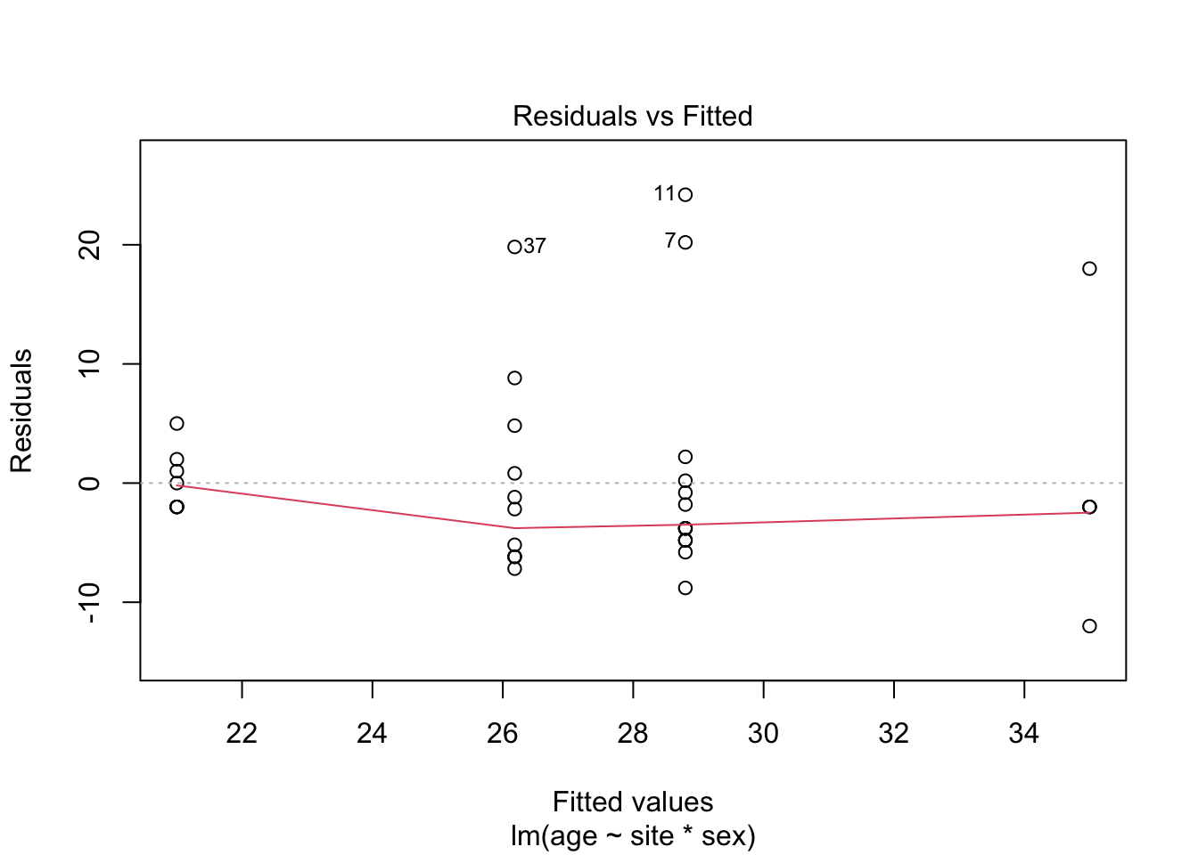
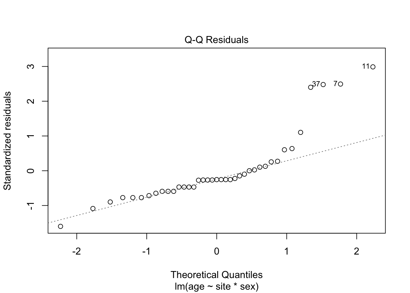
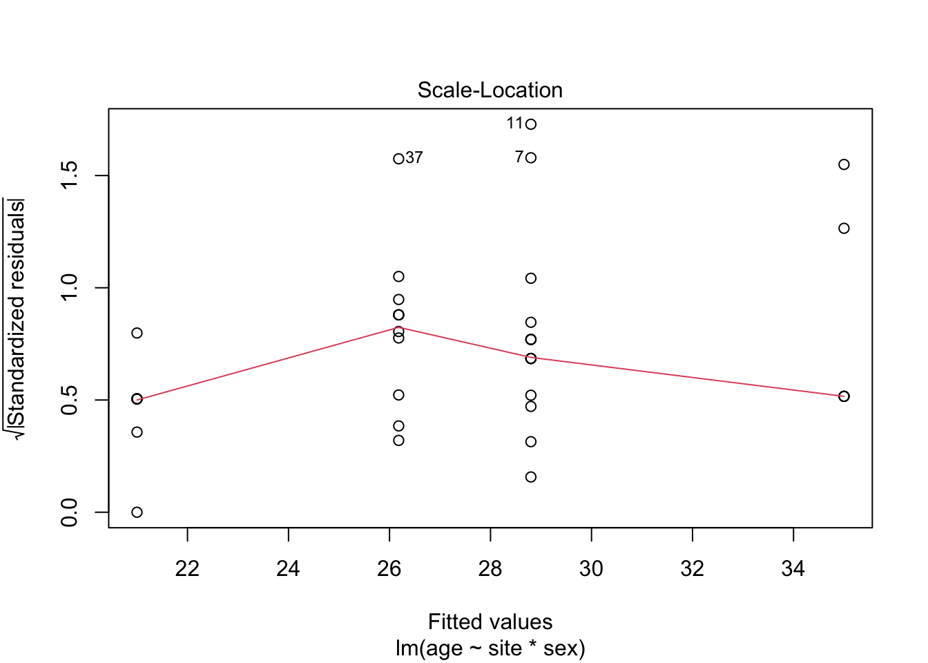
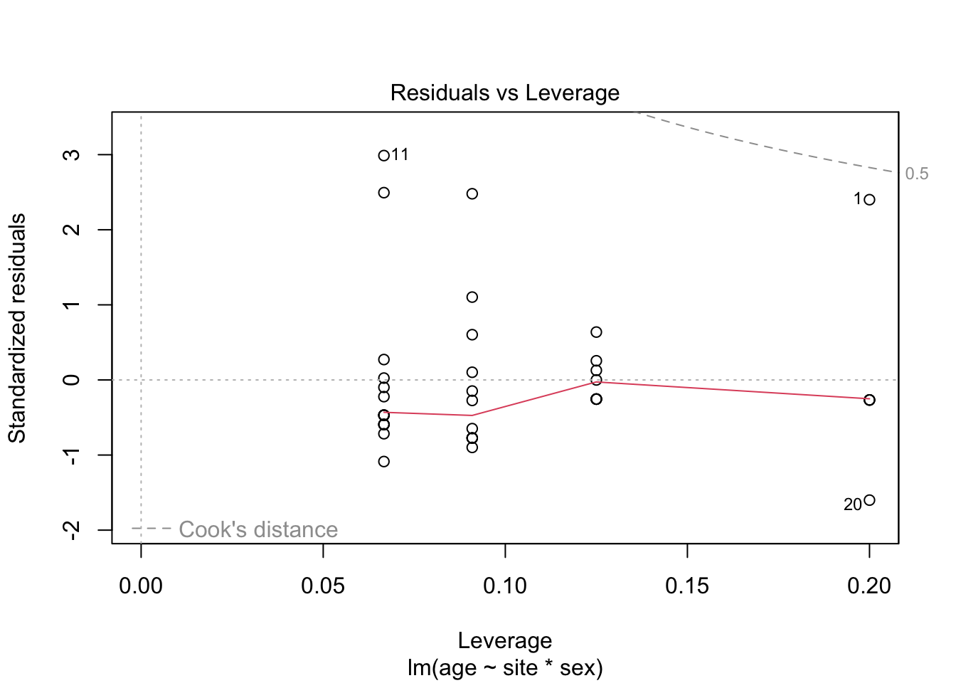
plot(model_age2)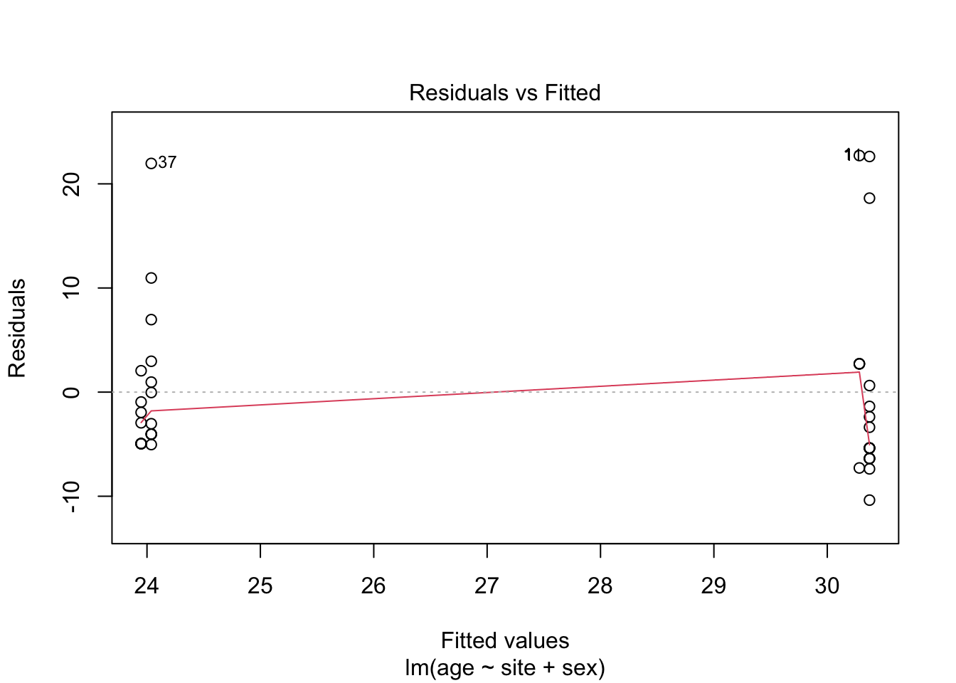
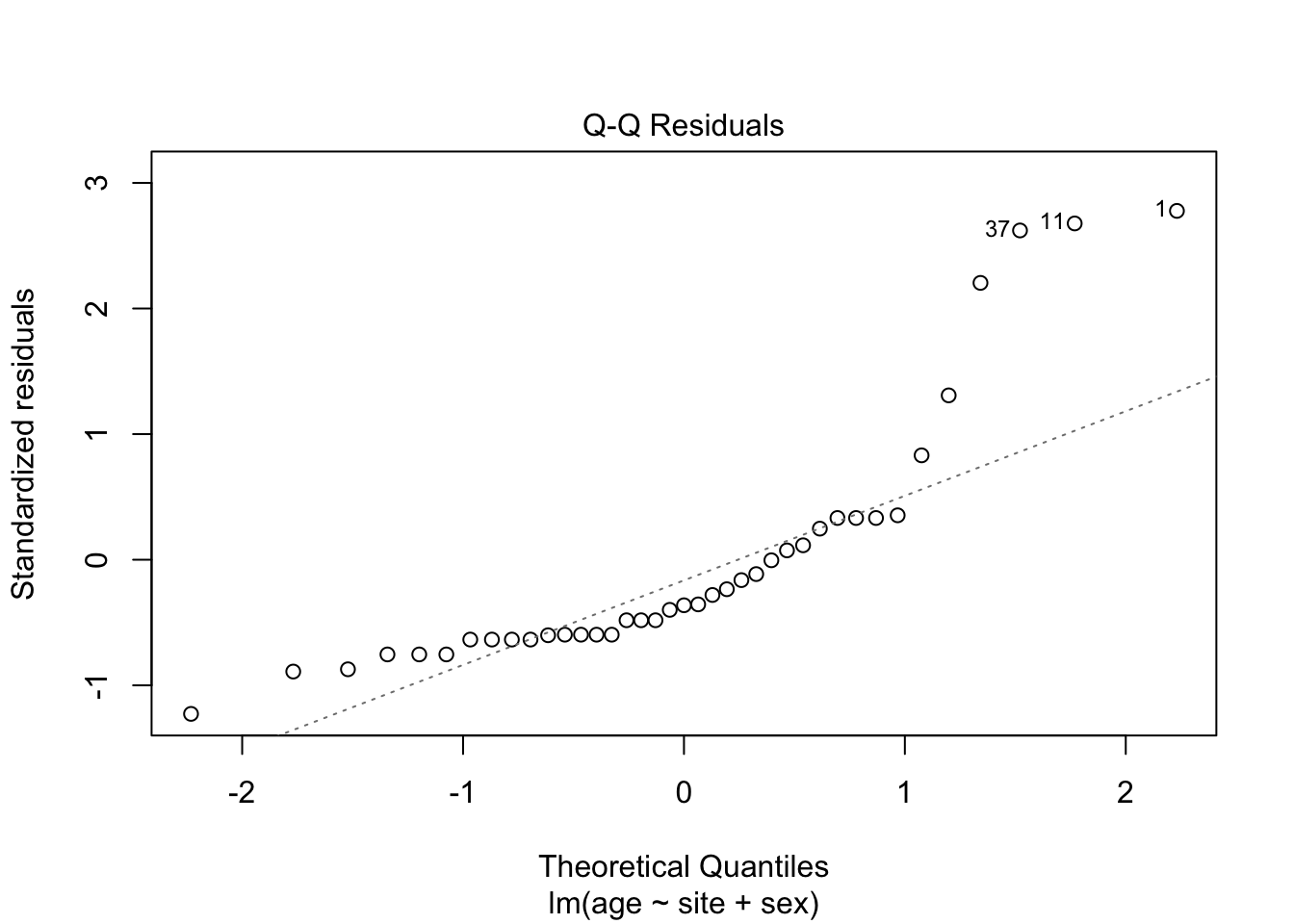

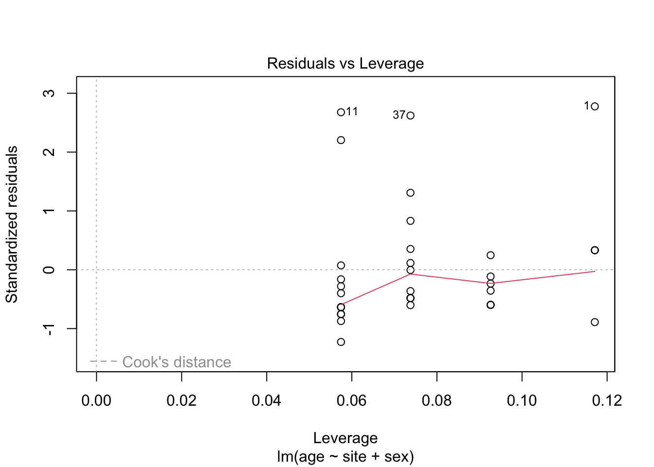
There is some evidence that age is different in the two sites, with participants about 6 years older in Switzerland compared to Malaysia. There is no significant difference in sex, nor is there a difference in sex between the sites (interaction of sex*site). Because of the significant age difference, age is a confounder for a comparison between the sites, with sparse coverage of the age range. Thus we will not explore how age affects light exposure in general, but rather whether age-differences from the site-mean affect light exposure. These results will have to be taken very tentative, as data is sparse.
form_age <- log10(MEDI) ~ site +                      # site main effect
            s(age_cs, by = site, k = 6) +                         # overall age trend
            te(Time, age_cs, by = site,                # age × time within site
               bs = c("cc", "tp"), k = c(12, 5)) +
            s(Id, bs = "re")                          # random intercepts
knots_day <- list(Time = c(0, 24))

m_age <- bam(
  form_age,
  data = le_data,
  knots = knots_day,
  select = TRUE,
  samfrac = 0.1,
  discrete = FALSE,
  nthreads = 4,
  control = list(nthreads = 4)
)

#Model performance
AICs <-
AIC(m_age, sex_model0)
AICs
df AIC
m_age 139.56297 4482533
sex_model0 59.97069 4516271appraise(m_age)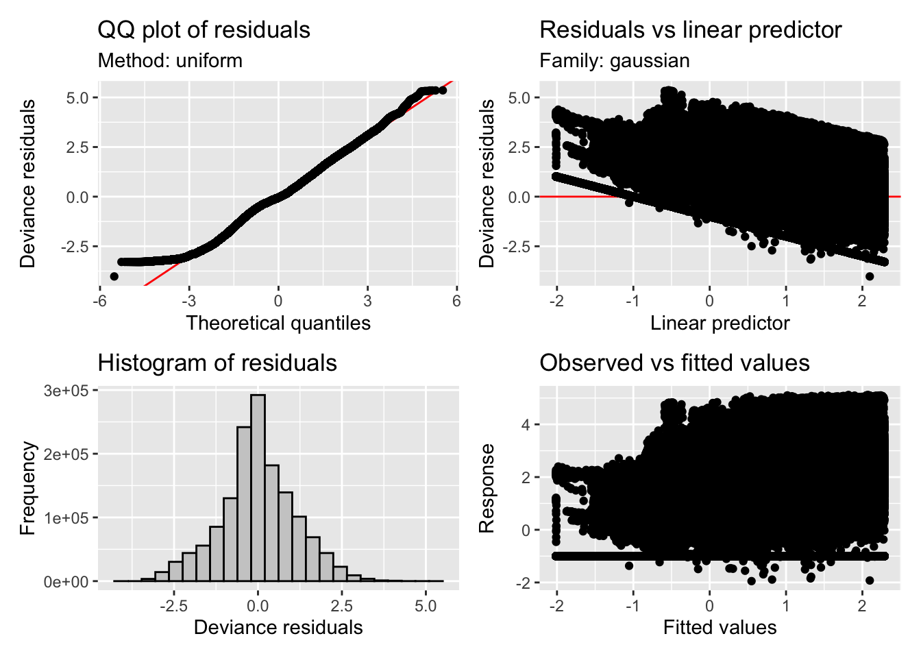
age_model_sum <-
summary(m_age)
age_model_sum
Family: gaussian
Link function: identity

Formula:
log10(MEDI) ~ site + s(age_cs, by = site, k = 6) + te(Time, age_cs,
    by = site, bs = c("cc", "tp"), k = c(12, 5)) + s(Id, bs = "re")

Parametric coefficients:
                Estimate Std. Error t value Pr(>|t|)
(Intercept)      0.44348    0.08006   5.539 3.04e-08 ***
siteswitzerland  0.03514    0.10638   0.330    0.741
---
Signif. codes:  0 '***' 0.001 '**' 0.01 '*' 0.05 '.' 0.1 ' ' 1

Approximate significance of smooth terms:
                                   edf Ref.df     F p-value
s(age_cs):sitemalaysia           1.530      5  5206 0.00460 **
s(age_cs):siteswitzerland        1.342      5  5950 0.00122 **
te(Time,age_cs):sitemalaysia    50.624     54  7593 < 2e-16 ***
te(Time,age_cs):siteswitzerland 50.248     54 16437 < 2e-16 ***
s(Id)                           32.701     37  1778 < 2e-16 ***
---
Signif. codes:  0 '***' 0.001 '**' 0.01 '*' 0.05 '.' 0.1 ' ' 1

R-sq.(adj) =  0.467   Deviance explained = 46.7%
fREML = 2.2417e+06 Scale est. = 1.236 n = 1469740draw(m_age, select = 1:2, residuals = FALSE) & theme_minimal()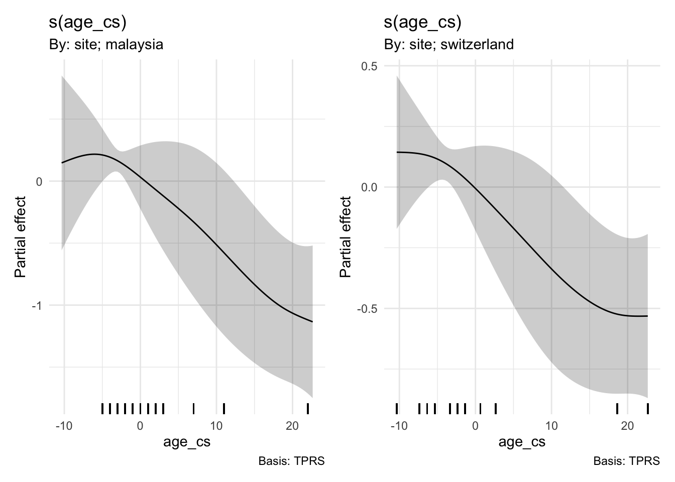
draw(m_age,
     select = 3:4,
     residuals = FALSE,
     rug = FALSE
     ) & theme_minimal()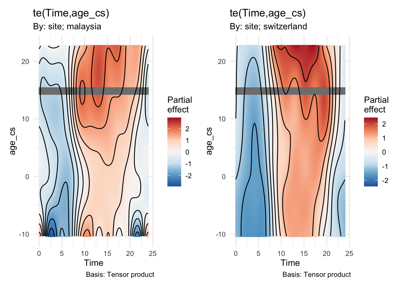
plot_diff(m_age,
          view = "Time",
          rm.ranef = "s(Id)",
          cond = list(site = "malaysia"),
          comp = list(age_cs = c(-5, 0)),
          sim.ci = TRUE)
Summary:
* site : factor; set to the value(s): malaysia.
* Time : numeric predictor; with 200 values ranging from 0.000000 to 23.983333.
* Id : factor; set to the value(s): ID07. (Might be canceled as random effect, check below.)
* NOTE : The following random effects columns are canceled: s(age_cs):sitemalaysia,s(age_cs):siteswitzerland,te(Time,age_cs):sitemalaysia,te(Time,age_cs):siteswitzerland,s(Id)
* Simultaneous 95%-CI used :
Critical value: 2.099
Proportion posterior simulations in pointwise CI: 1 (10000 samples)
Proportion posterior simulations in simultaneous CI: 1 (10000 samples)
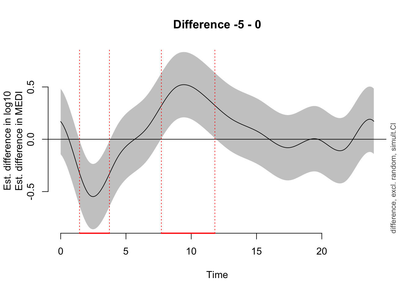
Time window(s) of significant difference(s):
    1.446231 - 3.736097
7.713233 - 11.810888plot_diff(m_age,
view = "Time",
rm.ranef = "s(Id)",
cond = list(site = "switzerland"),
comp = list(age_cs = c(-5, 0)),
sim.ci = TRUE)Summary:
* site : factor; set to the value(s): switzerland.
* Time : numeric predictor; with 200 values ranging from 0.000000 to 23.983333.
* Id : factor; set to the value(s): ID07. (Might be canceled as random effect, check below.)
* NOTE : The following random effects columns are canceled: s(age_cs):sitemalaysia,s(age_cs):siteswitzerland,te(Time,age_cs):sitemalaysia,te(Time,age_cs):siteswitzerland,s(Id)
* Simultaneous 95%-CI used :
Critical value: 2.108
Proportion posterior simulations in pointwise CI: 1 (10000 samples)
Proportion posterior simulations in simultaneous CI: 1 (10000 samples)
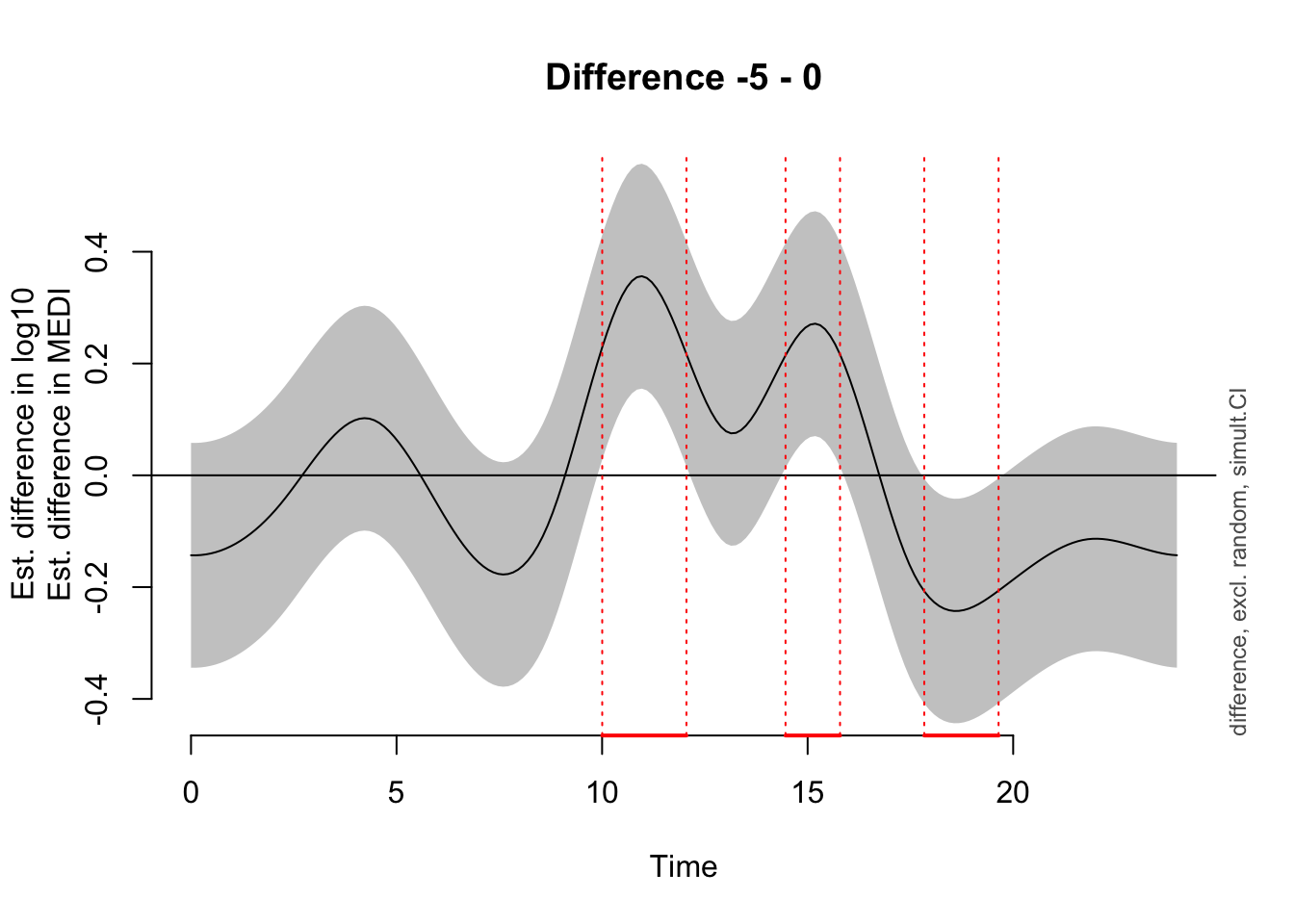
Time window(s) of significant difference(s):
    10.003099 - 12.051926
    14.462312 - 15.788023
17.836851 - 19.644640plot_diff(m_age,
view = "Time",
rm.ranef = "s(Id)",
# cond = list(site = "switzerland"),
comp = list(age_cs = c(-6, 0), site = c("switzerland", "malaysia")),
sim.ci = TRUE)Summary:
* Time : numeric predictor; with 200 values ranging from 0.000000 to 23.983333.
* Id : factor; set to the value(s): ID07. (Might be canceled as random effect, check below.)
* NOTE : The following random effects columns are canceled: s(age_cs):sitemalaysia,s(age_cs):siteswitzerland,te(Time,age_cs):sitemalaysia,te(Time,age_cs):siteswitzerland,s(Id)
* Simultaneous 95%-CI used :
Critical value: 2.097
Proportion posterior simulations in pointwise CI: 1 (10000 samples)
Proportion posterior simulations in simultaneous CI: 1 (10000 samples)
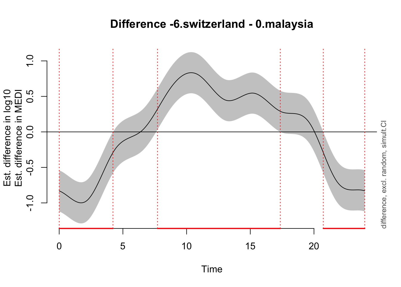
Time window(s) of significant difference(s):
    0.000000 - 4.218174
    7.713233 - 17.354774
20.729313 - 23.983333plot_diff(m_age,
view = "Time",
rm.ranef = "s(Id)",
cond = list(site = "malaysia"),
comp = list(age_cs = c(0, 20)),
sim.ci = TRUE)Summary:
* site : factor; set to the value(s): malaysia.
* Time : numeric predictor; with 200 values ranging from 0.000000 to 23.983333.
* Id : factor; set to the value(s): ID07. (Might be canceled as random effect, check below.)
* NOTE : The following random effects columns are canceled: s(age_cs):sitemalaysia,s(age_cs):siteswitzerland,te(Time,age_cs):sitemalaysia,te(Time,age_cs):siteswitzerland,s(Id)
* Simultaneous 95%-CI used :
Critical value: 2.142
Proportion posterior simulations in pointwise CI: 1 (10000 samples)
Proportion posterior simulations in simultaneous CI: 1 (10000 samples)
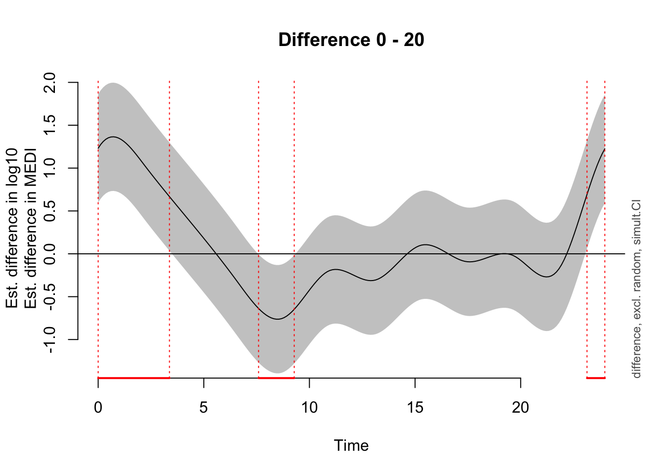
Time window(s) of significant difference(s):
    0.000000 - 3.374539
    7.592714 - 9.279983
23.139698 - 23.983333plot_diff(m_age,
view = "Time",
rm.ranef = "s(Id)",
cond = list(site = "switzerland"),
comp = list(age_cs = c(0, 20)),
sim.ci = TRUE)Summary:
* site : factor; set to the value(s): switzerland.
* Time : numeric predictor; with 200 values ranging from 0.000000 to 23.983333.
* Id : factor; set to the value(s): ID07. (Might be canceled as random effect, check below.)
* NOTE : The following random effects columns are canceled: s(age_cs):sitemalaysia,s(age_cs):siteswitzerland,te(Time,age_cs):sitemalaysia,te(Time,age_cs):siteswitzerland,s(Id)
* Simultaneous 95%-CI used :
Critical value: 2.099
Proportion posterior simulations in pointwise CI: 1 (10000 samples)
Proportion posterior simulations in simultaneous CI: 1 (10000 samples)
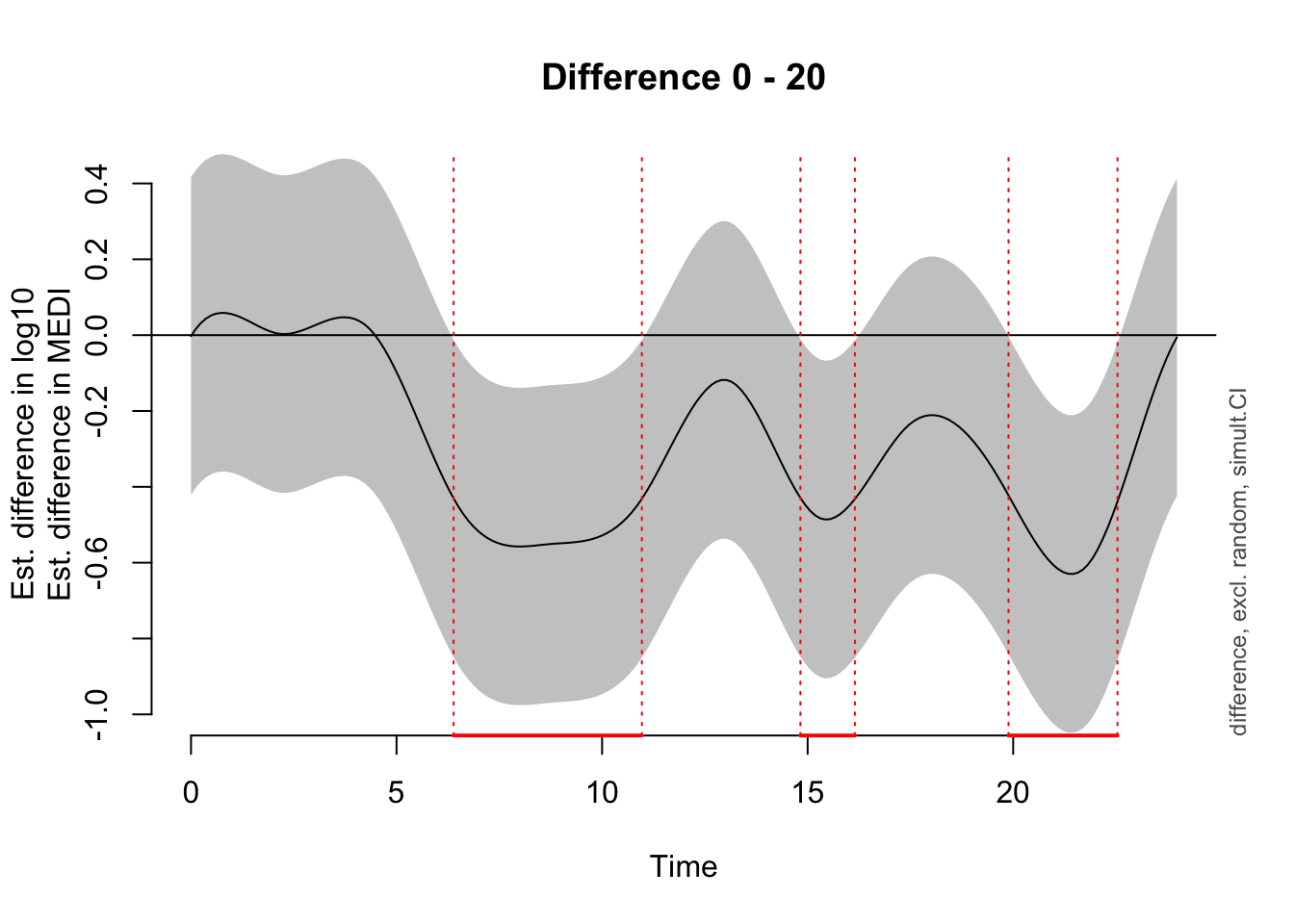
Time window(s) of significant difference(s):
    6.387521 - 10.967253
    14.823869 - 16.149581
    19.885678 - 22.537102
Results will be divided depending on where is comparatively good coverage of data, and sparse. All of these results should be interpreted tentatively. Good coverage:
There is some evidence that younger participants (average - 5 years) in Malaysia have brighter mornings and darker nights, whereas younger participants in Switzerland have brighter times before and after noon, as well as darker evenings.
Even when corrected for the age difference, the overall difference pattern between the sites remain: Participants in switzerland exhibit brighter days, particularly in the morning, and darker nights.
Sparse coverage:
- Older participants in both Malaysia and Switzerland seem to have brighter early mornings. Whereas participants in Malaysia exhibit darker nights, older swiss participants have brighter afternoons and evenings, each compared to their average age group.
7.3 Photoperiod duration
We explore the effect of photoperiod changes on light exposure patterns (in Switzerland)
le_data_swiss <-
  le_data |>
  filter(site == "switzerland") |>
  mutate(Datetime = with_tz(Datetime, tzs$switzerland)) |>
  add_photoperiod(coordinates$switzerland[2:1]) |>
  mutate(photoperiod = as.numeric(photoperiod) |> scale(scale = FALSE))

le_data_swiss |> pull(photoperiod) |> range()
[1] -2.466231 2.481652le_data_swiss |> extract_photoperiod(coordinates$switzerland[2:1]) |>
ggplot(aes(x = photoperiod)) + geom_histogram(binwidth = 30/60)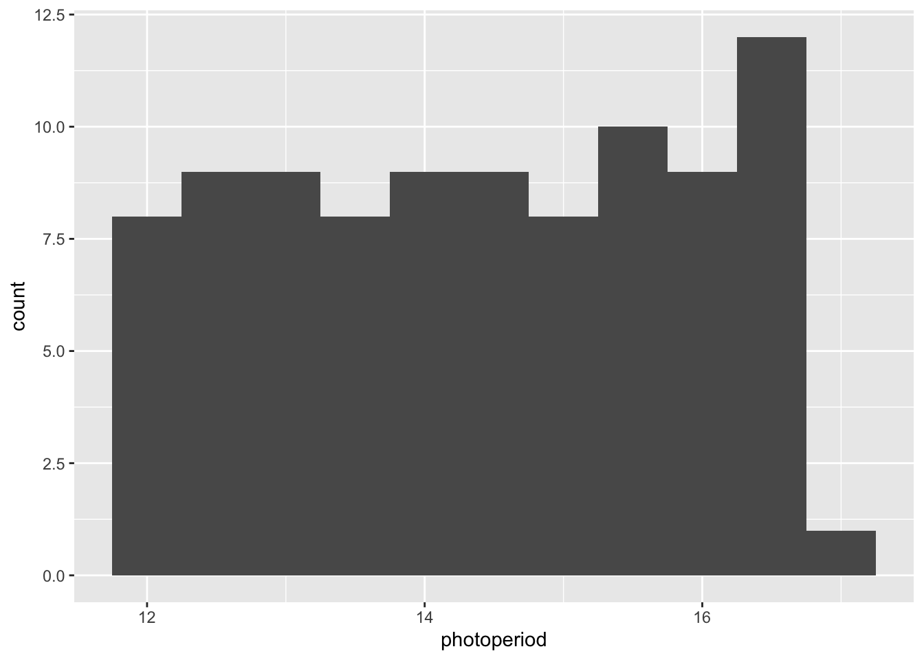
form_pp <- log10(MEDI) ~ photoperiod +
            te(Time, photoperiod,
               bs = c("cc", "tp"), k = c(10, 5)) +
            s(Id, bs = "re")
form_pp2 <- log10(MEDI) ~
            te(Time, photoperiod,
               bs = c("cc", "tp"), k = c(10, 5)) +
            s(Id, bs = "re")
form_pp0 <- log10(MEDI) ~
            te(Time,
               bs = c("cc"), k = c(10)) +
            s(Id, bs = "re")
knots_day <- list(Time = c(0, 24))

m_pp <- bam(
  form_pp,
  data = le_data_swiss,
  knots = knots_day,
  select = TRUE,
  samfrac = 0.1,
  discrete = FALSE,
  nthreads = 4,
  control = list(nthreads = 4)
)

m_pp2 <- bam(
  form_pp2,
  data = le_data_swiss,
  knots = knots_day,
  select = TRUE,
  samfrac = 0.1,
  discrete = FALSE,
  nthreads = 4,
  control = list(nthreads = 4)
)

m_pp0 <- bam(
  form_pp0,
  data = le_data_swiss,
  knots = knots_day,
  select = TRUE,
  samfrac = 0.1,
  discrete = FALSE,
  nthreads = 4,
  control = list(nthreads = 4)
)

#Model performance
AICs <-
AIC(m_pp, m_pp0, m_pp2)
AICs
df AIC
m_pp 64.76056 2323393
m_pp0 28.99263 2337187
m_pp2 64.76102 2323393appraise(m_pp)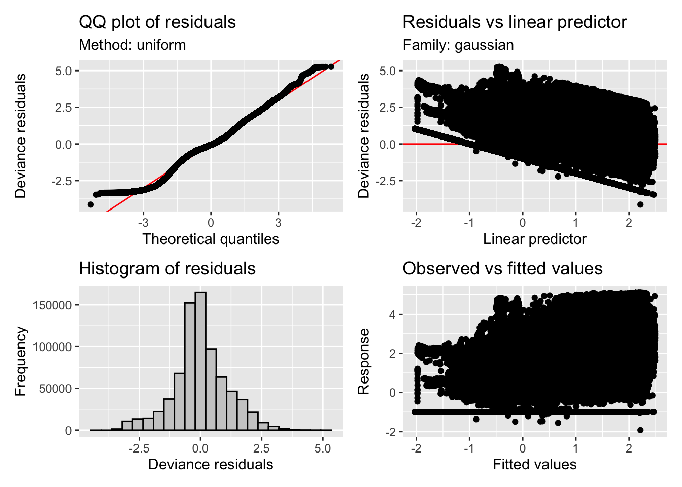
summary(m_pp2)
Family: gaussian
Link function: identity

Formula:
log10(MEDI) ~ te(Time, photoperiod, bs = c("cc", "tp"), k = c(10,
    5)) + s(Id, bs = "re")

Parametric coefficients:
            Estimate Std. Error t value Pr(>|t|)
(Intercept)  0.49241    0.07132   6.904 5.07e-12 ***
---
Signif. codes:  0 '***' 0.001 '**' 0.01 '*' 0.05 '.' 0.1 ' ' 1

Approximate significance of smooth terms:
                       edf Ref.df      F p-value
te(Time,photoperiod) 43.74     44 525647  <2e-16 ***
s(Id)                18.99     19   1953  <2e-16 ***
---
Signif. codes:  0 '***' 0.001 '**' 0.01 '*' 0.05 '.' 0.1 ' ' 1

R-sq.(adj) =   0.53   Deviance explained =   53%
fREML = 1.1619e+06 Scale est. = 1.2174 n = 765617draw(m_pp2, select = 1, rug = FALSE)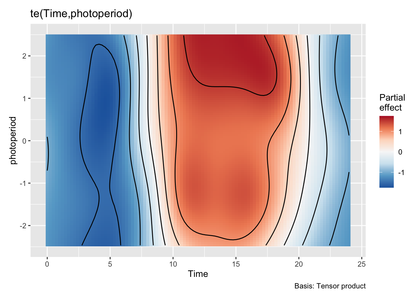
sm <-
  smooth_estimates(m_pp2, n = 24*4) |> add_confint()

pp_plot_model <-
sm |>
  filter(.smooth == "te(Time,photoperiod)") |>
  ggplot() +
  geom_tile(aes(x = Time, y = photoperiod, fill = (.estimate))) +
  geom_vline(xintercept = c(4,8, 12, 16, 20), lty = 2)+
  theme_cowplot() +
  labs(y = "Diff. photoperiod from average (hours)", x = "Time (hours)", fill = "Estimate of\nlog10(melEDI)") +
  scale_fill_viridis_c(
  ) +
  scale_x_continuous(breaks = seq(0, 24, by = 4))+
  coord_cartesian(xlim = c(0,24), expand = FALSE)

pp_plot_data <-
le_data_swiss |>
  add_photoperiod(coordinates$switzerland[2:1], overwrite = TRUE) |>
  mutate(photoperiod = as.numeric(photoperiod) %/% (5/60) * (5/60),
         Time = Time %/% (5/60) * (5/60)
         ) |>
  summarize(.by = c(photoperiod, Time), MEDI = median(MEDI)) |>
  ggplot(aes(x= Time, y = photoperiod, fill = MEDI-0.1)) +
  geom_tile()+
  geom_vline(xintercept = c(4,8, 12, 16, 20), lty = 2)+
  labs(y = "Photoperiod (hours)", x = "Time (hours)", fill = "mel EDI (lx)") +
  theme_cowplot()+
  scale_fill_viridis_b(trans = "symlog", breaks = c(0, 10^(0:3)), option = "E",
                       labels = c("0", "1", "10", "100", "1000")) +
  scale_x_continuous(breaks = seq(0, 24, by = 4))+
  coord_cartesian(xlim = c(0,24), expand = FALSE)

pp_plot_model + pp_plot_data + plot_layout(guides = "collect")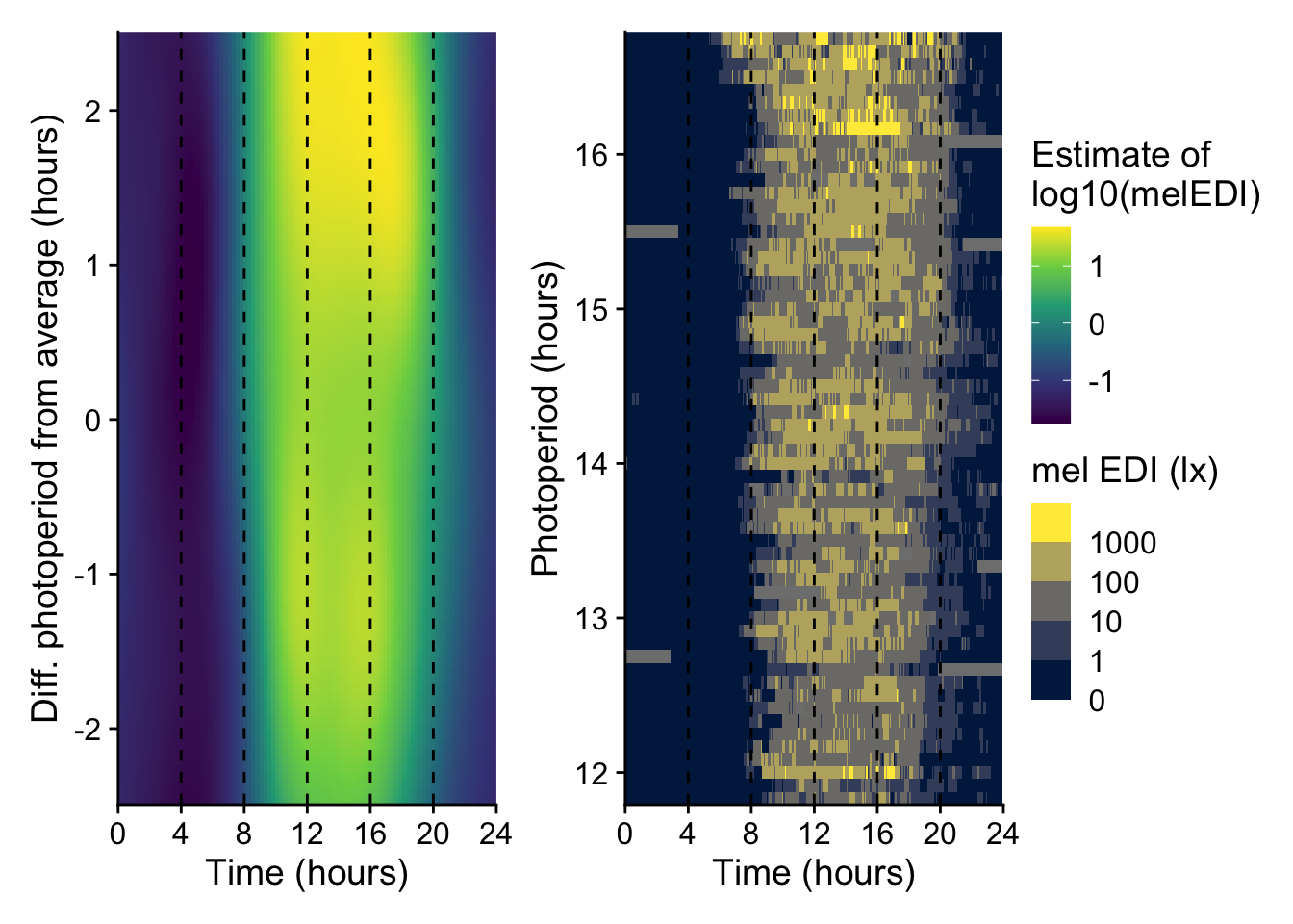
ggsave("figures/Figure_S4.pdf",
       width = 17, height = 7, units = "cm", scale = 1.6)

gam.check(m_pp2)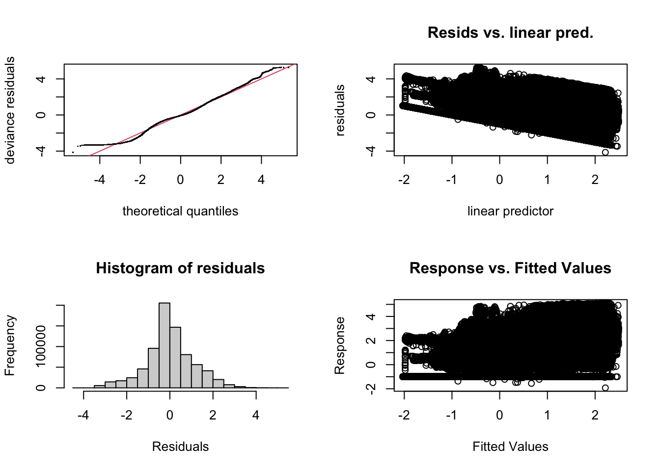
Method: fREML   Optimizer: perf newton
full convergence after 17 iterations.
Gradient range [-0.002184891,0.002181797]
(score 1161887 & scale 1.217384).
Hessian positive definite, eigenvalue range [0.5017434,382808].
Model rank =  65 / 65

Basis dimension (k) checking results. Low p-value (k-index<1) may
indicate that k is too low, especially if edf is close to k'.

                       k'  edf k-index p-value
te(Time,photoperiod) 44.0 43.7    0.94  <2e-16 ***
s(Id)                20.0 19.0      NA      NA
---
Signif. codes:  0 '***' 0.001 '**' 0.01 '*' 0.05 '.' 0.1 ' ' 1
From the model results we can see that for the light exposure overall, photoperiod has no mere parametric influence, but rather influences the pattern. Both raw data and modelled representation show a gradual extension towards longer exposure into the evening, while there is moderate extension into the morning. In all (photoperiod) cases, there are two pronounced high-points during the day, one around noon, and the second in the afternoon around 4 pm. Due to the noise in the data, this is better reflected in the model representation.
7.4 Chronotype effect
In this section, we look into the effect of chronotype on the timing of light exposure. Specifically the mean timing of light exposure above 250 lx melanopic EDI (MLiT250). We did not assess chronotype directly. However, questions in the PSQI refer to the timing of sleep, which can be used to calculate the mid-sleep.
#combined dataset
psqi_switzerland <-
  psqi_switzerland |>
                  rename(Id = code,
                         psqi_01_corrected = psqi_q1_bedtime,
                         psqi_02_corrected = psqi_q2_sleeptime,
                         psqi_03_corrected = psqi_q3_getuptime,
                         )
#calculate chronotype
CT_combined <-
  join_datasets(psqi_malaysia,
                psqi_switzerland,
                add.origin = TRUE,
                Datetime.column = Day
                ) |>
  select(dataset, Id, Day, ends_with("_corrected")) |>
    filter(Day == 31 | Id %in% c("1990ZEZA", "1996VILE")) |>
    mutate(site = str_extract(dataset, "(?<=psqi_).*")) |>
    select( -psqi_04_corrected, -dataset) |>
    drop_na() |>
    mutate(Sonset = hms::as_hms(psqi_01_corrected + dminutes(psqi_02_corrected)),
           Soffset = psqi_03_corrected,
           MS = Soffset - Sonset,
           MS = ifelse(MS <= 0, MS + ddays(1), MS),
           MS = MS/2,
           MS = (MS + ifelse((MS + Sonset) > 24*60*60,
                               Sonset - ddays(1),
                               Sonset)
                  ) |> hms::as_hms(),
           Chronotype = cut(MS |> as.numeric(),
                            breaks = c(0, 3*60*60, 4*60*60, 24*60*60),
                            labels = c("early", "intermediate", "late")
                            )
           )

#correct for Id values in Switzerland
CT_combined <-
  CT_combined |>
    left_join(conv_switzerland, by = join_by(Id == Code)) |>
    mutate(Id = coalesce(ID, Id)) |>
    select(-ID)

CT_combined |>
  mutate(site = str_to_title(site)) |>
  ggplot(aes(x = site, y = MS)) +
  geom_boxplot(aes(fill = site)) +
  geom_jitter(width = 0.1, alpha = 0.25) +
  theme_cowplot() +
  scale_fill_jco() +
  guides(fill = "none") +
  labs(y = "Chronotype (Mid-sleep, HH:MM)", x = "Site") +
  scale_y_time(labels = \(x) strftime(x, format = "%H:%M"))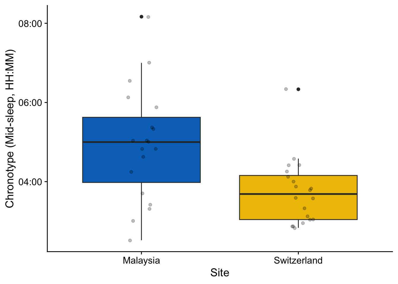
ggsave("figures/Figure_S5.pdf",
       width = 7, height = 7, units = "cm", scale = 1.6)

CT_model <- lm(as.numeric(MS) ~ site, data = CT_combined)
summary(CT_model)
Call:
lm(formula = as.numeric(MS) ~ site, data = CT_combined)

Residuals:
    Min      1Q  Median      3Q     Max
-8735.5 -2527.5   172.5  1681.0 11589.5

Coefficients:
                Estimate Std. Error t value Pr(>|t|)
(Intercept)      17810.5      959.3  18.566  < 2e-16 ***
siteswitzerland  -4333.0     1339.6  -3.234  0.00257 **
---
Signif. codes:  0 '***' 0.001 '**' 0.01 '*' 0.05 '.' 0.1 ' ' 1

Residual standard error: 4182 on 37 degrees of freedom
Multiple R-squared:  0.2204,    Adjusted R-squared:  0.1994
F-statistic: 10.46 on 1 and 37 DF,  p-value: 0.002567
CT_combined |>
summarize(mean = mean(MS) |> round() / 3600,
sd = sd(MS)|> round() / 3600,
.by = site)# A tibble: 2 × 3
site mean sd
<chr> <drtn> <dbl>
1 malaysia 4.947500 secs 1.43
2 switzerland 3.743889 secs 0.838extract_data <-
data$malaysia |> group_by(Id, Day) |> filter(Datetime == min(Datetime))
solar_noon(coordinates = coordinates$malaysia[2:1], dates = extract_data$Day, tz = tzs$malaysia) |>
add_Time_col(Datetime.colname = solar.noon) |>
summarize(mean_ml = (mean(Time)/3600 )|> as.numeric()) mean_ml
1 13.09807extract_data <-
data$switzerland |> group_by(Id, Day) |> filter(Datetime == min(Datetime))
solar_noon(coordinates = coordinates$switzerland[2:1], dates = extract_data$Day, tz = tzs$switzerland) |>
add_Time_col(Datetime.colname = solar.noon) |>
summarize(mean_ml = (mean(Time)/3600 )|> as.numeric()) mean_ml
1 13.46677Two participants in Switzerland (1990ZEZA and 1996VILE) only have a PSQI filled in for the first day, but not the last of the trial. For those two, the first day is used. Chronotypes differ significantly between the two sites, with earlier chronotypes in Switzerland (mid-sleep ~5:00a.m. in Malaysia, and about 1:12 hours earlier in Switzerland, i.e., ~3:48a.m.).
MLiT250 <-
le_data |>
  group_by(site, Id, Day) |>
  mutate(Time = (Time * 3600) |> hms::as_hms()) |>
  summarize(
    timing_above_threshold(MEDI,
                           Time,
                           "above",
                           250,
                           na.rm = TRUE,
                           as.df = TRUE),
    .groups = "drop_last"
    ) |>
  left_join(CT_combined, by = c("site", "Id")) |>
  select(site, Id, mean_timing_above_250, MS, Chronotype, Day.x) |>
  mutate(MLiT250 = hms::as_hms(mean_timing_above_250))
MLiT250_rad <-
MLiT250 |>
mutate(across(c(MS, MLiT250), \(x) as.numeric(x) %% 86400),
across(c(MS, MLiT250), \(x) circular(
x / 86400 * 2 * pi, type = "angles", units = "radians",
template = "clock24"
))
)
cor.values <-
MLiT250_rad |>
group_by(site) |>
reframe(cor = as.tibble(cor.circular(MLiT250, MS, test = TRUE))) |>
unnest(cor) |>
mutate(site = site |> str_to_title(),
p.value = p.value |> gtsummary::label_style_pvalue(2)(),
r = cor |> round(2)) |>
select(-cor, -statistic)
cor.values |> gt() |> tab_header("(Circular) correlation of MLiT250 and chronotype")| (Circular) correlation of MLiT250 and chronotype | ||
|---|---|---|
| site | p.value | r |
| Malaysia | <0.001 | 0.22 |
| Switzerland | 0.27 | 0.05 |
model_CT0 <- lmer(MLiT250 ~ site + (1|Id), data = MLiT250_rad)
model_CT1 <- lmer(MLiT250 ~ MS + site + (1|Id), data = MLiT250_rad)
model_CT2 <- lmer(MLiT250 ~ MS*site + (1|Id), data = MLiT250_rad)
anova(model_CT0, model_CT1, model_CT2)
Data: MLiT250_rad
Models:
model_CT0: MLiT250 ~ site + (1 | Id)
model_CT1: MLiT250 ~ MS + site + (1 | Id)
model_CT2: MLiT250 ~ MS * site + (1 | Id)
npar AIC BIC logLik -2*log(L) Chisq Df Pr(>Chisq)
model_CT0 4 1360.1 1379.5 -676.04 1352.1
model_CT1 5 1356.0 1380.3 -673.00 1346.0 6.0709 1 0.01374 *
model_CT2 6 1357.1 1386.3 -672.57 1345.1 0.8676 1 0.35161
---
Signif. codes: 0 '***' 0.001 '**' 0.01 '*' 0.05 '.' 0.1 ' ' 1model_CT1 |> summary()Linear mixed model fit by REML ['lmerMod']
Formula: MLiT250 ~ MS + site + (1 | Id)
Data: MLiT250_rad
REML criterion at convergence: 1358.5
Scaled residuals:
Min 1Q Median 3Q Max
-4.4442 -0.5983 -0.0391 0.5486 4.2955
Random effects:
Groups Name Variance Std.Dev.
Id (Intercept) 0.01816 0.1348
Residual 0.23000 0.4796
Number of obs: 956, groups: Id, 39
Fixed effects:
Estimate Std. Error t value
(Intercept) 3.23604 0.12446 26.001
MS 0.22492 0.09075 2.478
siteswitzerland 0.22572 0.06111 3.694
Correlation of Fixed Effects:
(Intr) MS
MS -0.950
sitswtzrlnd -0.645 0.470CT_P1 <-
MLiT250 |>
mutate(site = site |> str_to_title()) |>
ggplot(aes(x=MS, y = MLiT250)) +
geom_point(alpha = 0.5) +
geom_smooth(aes(col = site, fill = site), method = "lm") +
facet_wrap(~site) +
geom_text(data = cor.values,
aes(label = paste0("r: ", r, ", p: ", p.value),
x = 8*60*60,
y = 22*60*60,
hjust = 1)
) +
theme_cowplot() +
scale_fill_jco() +
scale_color_jco() +
scale_y_time(labels = \(x) strftime(x, format = "%H:%M")) +
scale_x_time(labels = \(x) strftime(x, format = "%H:%M")) +
guides(col = "none", fill = "none") +
labs(x = "Chronotype (mid-sleep, HH:MM)",
y = "Mean timing of light (MLiT) \nabove 250lx mel EDI (HH:MM)")
CT_P2 <-
MLiT250 |>
mutate(site = site |> str_to_title()) |>
ggplot(aes(x=Chronotype, y = MLiT250)) +
geom_violin(aes(
alpha = Chronotype), fill = "grey", col = "grey", linewidth = 0.1) +
scale_fill_jco()+
guides(fill = "none", alpha = "none") +
geom_boxplot(width = 0.25, aes(fill = site), linewidth = 0.35) +
# geom_jitter(width = 0.05, alpha = 0.1) +
scale_y_time(labels = \(x) strftime(x, format = "%H:%M")) +
facet_wrap(~site) +
labs(x = "Chronotype (based on mid-sleep)",
y = "Mean timing of light (MLiT) \nabove 250lx mel EDI (HH:MM)",
caption = "Intermediate: 3 a.m. ≤ mid-sleep ≤ 4 a.m") +
theme_cowplot()
# CT_P1 / CT_P2 + plot_layout(axes = "collect")
CT_P1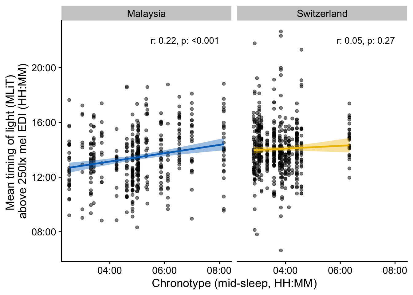
ggsave("figures/Figure_3.pdf",
       width = 9, height = 6, units = "cm", scale = 1.6)

 MLiT250 <-
  MLiT250 |> mutate(across(where(hms::is.hms), \(x) as.numeric(x)/3600))

CT_model <- lmerTest::lmer(MLiT250 ~ MS*site + (1|Id), data = MLiT250)

CT_model |> summary()
Linear mixed model fit by REML. t-tests use Satterthwaite's method [
lmerModLmerTest]
Formula: MLiT250 ~ MS * site + (1 | Id)
Data: MLiT250
REML criterion at convergence: 3916.1
Scaled residuals:
Min 1Q Median 3Q Max
-4.4430 -0.5945 -0.0398 0.5485 4.2962
Random effects:
Groups Name Variance Std.Dev.
Id (Intercept) 0.2665 0.5162
Residual 3.3561 1.8320
Number of obs: 956, groups: Id, 39
Fixed effects:
Estimate Std. Error df t value Pr(>|t|)
(Intercept) 12.1182 0.5509 33.9304 21.998 <2e-16 ***
MS 0.2737 0.1066 33.3631 2.568 0.0149 *
siteswitzerland 1.5964 0.8687 32.3631 1.838 0.0753 .
MS:siteswitzerland -0.1793 0.2043 31.6975 -0.878 0.3867
---
Signif. codes: 0 '***' 0.001 '**' 0.01 '*' 0.05 '.' 0.1 ' ' 1
Correlation of Fixed Effects:
(Intr) MS stswtz
MS -0.963
sitswtzrlnd -0.634 0.611
MS:stswtzrl 0.502 -0.522 -0.963Chronotype is significantly correlated with the mean timing of light exposure above 250 lx melanopic EDI (MLiT250) in Malaysia, but not Switzerland. The significant effect size is small (r = 0.22, p < 0.001). Per hour of increase in mid-sleep timing, MLiT250 increases about 16.4 minutes.
7.5 Brown recommendations
In this section, we look into the compliance to the Brown recommendations for healthy lighting. We use the sleep-wake-data derived from the PSQI as a proxy for day-specific sleep times, and calculate the compliance per site, and also per site and time of day.
sleep_combined <-
  CT_combined |>
  mutate(Sonset = ifelse(Sonset >= 24*60*60, Sonset - 24*60*60, Sonset) |>
           hms::as_hms()) |>
  select(site, Id, Sonset, Soffset) |>
  rename(sleep = Sonset, wake = Soffset) |>
  pivot_longer(names_to = "State",
               cols = c(sleep, wake),
               values_to = "Time") |>
  mutate(Id = fct_relabel(Id, \(x) str_remove(x, "ID|MY0")),
         Id = factor(Id, levels = sprintf("%02d", 1:20)),
         site = str_to_title(site)) |>
  arrange(site, Id)


sleep_data <-
data_combined |>
  select(site, Id, Day) |>
  distinct() |>
  left_join(sleep_combined, by = c("site", "Id"), relationship = "many-to-many")

sleep_data <-
sleep_data |>
  group_by(site) |>
  mutate(Datetime = lubridate::as_datetime(paste(Day, Time))) |>
  select(site, Id, Datetime, State) |>
  arrange(site, Id, Datetime)

sleep_intervals <-
  sleep_data |>
  group_by(site, Id) |>
  sc2interval()
Brown_intervals <-
sleep_intervals |>
group_by(site, Id) |>
sleep_int2Brown() |>
drop_na() |>
mutate(Id = interaction(site, Id)) |>
mutate(start = int_start(Interval), end = int_end(Interval)) |>
ungroup(site) |>
select(-site, -Interval) brown_data <-
data_combined |> select(site, Id, Datetime, MEDI, dusk, dawn) |>
mutate(Id = interaction(site, Id)) |>
group_by(Id) |>
add_states(Brown_intervals) |>
# interval2state(Brown_intervals, State.colname = State.Brown, overwrite = TRUE) |>
add_Time_col()state_compliance <-
brown_data |>
Brown2reference() |>
drop_na(State.Brown) |>
group_by(site, State.Brown, .add = TRUE) |>
durations(Reference.check, show.missing = TRUE, FALSE.as.NA = TRUE) |>
mutate(
compliance = (duration/total),
site = str_to_title(site)
) |>
ungroup(Id) |>
drop_na() |>
summarize(across(-Id, mean), .groups = "drop") |>
mutate(across(c(duration, missing, total), as.duration),
compliance = compliance |> scales::percent(2)) |>
rename(compliant = duration,
`non-compliant` = missing,
) |>
group_by(State.Brown)
overall_compliance <-
state_compliance |>
group_by(site) |>
summarize(across(c(compliant, `non-compliant`, total),
\(x) sum(x) |> as.duration())) |>
mutate(compliance = (compliant/total) |> scales::percent(),
State.Brown = "overall")
compliance_table <-
rbind(state_compliance, overall_compliance) |>
mutate(State.Brown = str_to_title(State.Brown)) |>
select(site, State.Brown, compliance) |>
pivot_wider(names_from = State.Brown, values_from = compliance) |>
gt(rowname_col = "site") |>
tab_header("Compliance to Brown recommendation for healthy light exposure") |>
tab_footnote(md("*Day* includes the time from wake until evening (recommendation ≥ 250lx mel EDI).<br>*Evening* starts three hours prior to sleep until sleep onset (recommendation ≤ 10lx mel EDI).<br>*Night* covers the sleep times (recommendation ≤ 1lx mel EDI).<br>*Overall* indicates the time-weighted average compliance."))
compliance_table| Compliance to Brown recommendation for healthy light exposure | ||||
|---|---|---|---|---|
| Day | Evening | Night | Overall | |
| Malaysia | 10% | 64% | 84% | 39% |
| Switzerland | 26% | 78% | 92% | 54% |
| Day includes the time from wake until evening (recommendation ≥ 250lx mel EDI). Evening starts three hours prior to sleep until sleep onset (recommendation ≤ 10lx mel EDI). Night covers the sleep times (recommendation ≤ 1lx mel EDI). Overall indicates the time-weighted average compliance. |
||||
compliance_table |>
gtsave("figures/Table_1.png")

compliance_table |>
gtsave("figures/Table_1.docx")
compliance_Plot1 <-
brown_data |>
Brown2reference() |>
mutate(
Reference.check = ifelse(Reference.check, "compliant", "non-compliant")
) |>
drop_na(Reference.check) |>
ggplot(aes(x= Time, after_stat(count), fill = (Reference.check) |> fct_rev())) +
# geom_density(position = "fill", linewidth = 0.25, bw = 1/12) +
geom_density(position = "fill", linewidth = 0.25, bw = 1/12) +
facet_wrap(~site) +
theme_cowplot() +
# scale_fill_viridis_d(option = "A") +
# guides(fill = "none") +
labs(
x = "Local time (HH:MM)",
y = "Cumulative percentage (%)",
fill = "Compliance to recommendations") +
scale_y_continuous(labels = scales::label_percent()) +
scale_x_time(
breaks = seq(0, 24*60*60, by = 6*60*60),
labels = \(x) strftime(x, format = "%H:%M")
# labels = NULL
) +
# scale_x_continuous(
# breaks = seq(0, 24, by = 6),
# labels = \(x) sprintf("%2d:00", x)
# ) +
facet_wrap2( ~ site,
# switch = "y",
labeller = labeller(site = NA),
strip =
strip_themed(background_x = element_blank(),
text_x = element_blank())) +
theme(panel.spacing = unit(1.5, "lines"))
compliance_Plot2 <-
brown_data |>
Brown_cut(vector_labels = c("<1lx", "1 - 10lx", "10 - 250lx", "> 250lx")) |>
drop_na(state) |>
ggplot(aes(x= Time, after_stat(count), fill = fct_rev(state))) +
geom_density(position = "fill", col = NA, bw = 1/12) +
# facet_wrap(~site) +
scale_fill_manual(values = c("yellow", "darkgrey", "lightgrey", "black")) +
cowplot::theme_cowplot() +
# guides(fill = "none") +
labs(
x = "Local time (HH:MM)",
y = "Cumulative percentage (%)",
fill = "mel EDI (lx)") +
scale_y_continuous(labels = scales::label_percent()) +
scale_x_continuous(
breaks = seq(0, 24*60*60, by = 6*60*60),
labels = NULL
# labels = \(x) sprintf("%2d:00", x)
) +
facet_wrap2( ~ site,
# switch = "y",
# labeller = labeller(site = facet_names),
strip =
strip_themed(background_x = elem_list_rect(fill = pal_jco()(2)))) +
theme(panel.spacing = unit(1.5, "lines"))
# compliance_Plot3 <-
# brown_data |>
# drop_na(State.Brown) |>
# ggplot(aes(x= Time, after_stat(count), fill = fct_rev(State.Brown))) +
# geom_density(position = "fill", col = NA, bw = 1/12) +
# # facet_wrap(~site) +
# scale_fill_manual(values = c(night = "darkblue", evening = "lightyellow4", day = "skyblue2")) +
# cowplot::theme_cowplot() +
# # guides(fill = "none") +
# labs(
# x = "Local time (HH:MM)",
# y = "Cumulative percentage (%)",
# fill = "Brown states") +
# scale_y_continuous(labels = scales::label_percent()) +
# scale_x_time(
# breaks = seq(0, 24*60*60, by = 6*60*60),
# labels = NULL
# # labels = \(x) strftime(x, format = "%H:%M")
# ) +
# facet_wrap2( ~ site,
# # switch = "y",
# # labeller = labeller(site = facet_names),
# strip =
# strip_themed(background_x = element_blank(),
# text_x = element_blank())) +
# theme(panel.spacing = unit(1.5, "lines"))
compliance_Plot2 /
# compliance_Plot3 /
compliance_Plot1 +
plot_layout(axes = "collect") & theme(legend.position = "bottom")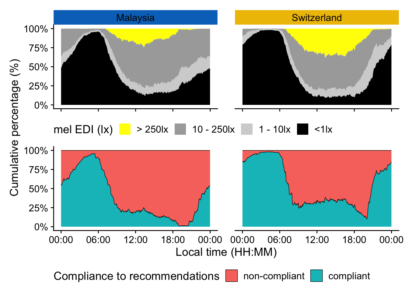
ggsave("figures/Figure_S6.pdf",
       width = 14, height = 12, units = "cm", scale = 1.6)
8 Session Info
sessionInfo()R version 4.5.0 (2025-04-11)
Platform: aarch64-apple-darwin20
Running under: macOS 26.1
Matrix products: default
BLAS: /Library/Frameworks/R.framework/Versions/4.5-arm64/Resources/lib/libRblas.0.dylib
LAPACK: /Library/Frameworks/R.framework/Versions/4.5-arm64/Resources/lib/libRlapack.dylib; LAPACK version 3.12.1
locale:
[1] en_US.UTF-8/en_US.UTF-8/en_US.UTF-8/C/en_US.UTF-8/en_US.UTF-8
time zone: Europe/Berlin
tzcode source: internal
attached base packages:
[1] stats graphics grDevices datasets utils methods base
other attached packages:
[1] sf_1.0-21 rnaturalearth_1.1.0 gratia_0.10.0
[4] rnaturalearthdata_1.0.0 webshot2_0.1.2 circular_0.5-1
[7] ggh4x_0.3.1 magick_2.8.7 ggtext_0.1.2
[10] ordinal_2023.12-4.1 labelled_2.14.1 itsadug_2.4.1
[13] plotfunctions_1.4 mgcv_1.9-3 nlme_3.1-168
[16] magrittr_2.0.3 lattice_0.22-7 broom.mixed_0.2.9.6
[19] lmerTest_3.1-3 lme4_1.1-37 Matrix_1.7-3
[22] here_1.0.1 legendry_0.2.2 suntools_1.0.1
[25] rlang_1.1.6 LightLogR_0.9.2 ggcorrplot_0.1.4.1
[28] ggsci_3.2.0 readxl_1.4.5 patchwork_1.3.1
[31] gtsummary_2.3.0 gt_1.0.0 cowplot_1.1.3
[34] lubridate_1.9.4 forcats_1.0.0 stringr_1.5.1
[37] dplyr_1.1.4 purrr_1.0.4 readr_2.1.5
[40] tidyr_1.3.1 tibble_3.2.1 ggplot2_3.5.2
[43] tidyverse_2.0.0
loaded via a namespace (and not attached):
[1] RColorBrewer_1.1-3 rstudioapi_0.17.1 jsonlite_2.0.0
[4] cardx_0.2.5 farver_2.1.2 nloptr_2.2.1
[7] rmarkdown_2.29 fs_1.6.6 ragg_1.4.0
[10] vctrs_0.6.5 minqa_1.2.8 base64enc_0.1-3
[13] janitor_2.2.1 htmltools_0.5.8.1 haven_2.5.5
[16] broom_1.0.8 cellranger_1.1.0 sass_0.4.10
[19] parallelly_1.45.1 KernSmooth_2.23-26 htmlwidgets_1.6.4
[22] commonmark_1.9.5 lifecycle_1.0.4 pkgconfig_2.0.3
[25] R6_2.6.1 fastmap_1.2.0 rbibutils_2.3
[28] future_1.67.0 snakecase_0.11.1 digest_0.6.37
[31] numDeriv_2016.8-1.1 furrr_0.3.1 ps_1.9.1
[34] rprojroot_2.0.4 warp_0.2.1 textshaping_1.0.1
[37] labeling_0.4.3 timechange_0.3.0 compiler_4.5.0
[40] proxy_0.4-27 bit64_4.6.0-1 withr_3.0.2
[43] backports_1.5.0 DBI_1.2.3 MASS_7.3-65
[46] ucminf_1.2.2 classInt_0.4-11 tools_4.5.0
[49] chromote_0.5.1 units_0.8-7 glue_1.8.0
[52] promises_1.3.3 gridtext_0.1.5 grid_4.5.0
[55] generics_0.1.4 isoband_0.2.7 gtable_0.3.6
[58] tzdb_0.5.0 class_7.3-23 websocket_1.4.4
[61] hms_1.1.3 xml2_1.3.8 utf8_1.2.6
[64] pillar_1.10.2 markdown_2.0 vroom_1.6.5
[67] later_1.4.2 splines_4.5.0 renv_1.0.11
[70] bit_4.6.0 tidyselect_1.2.1 knitr_1.50
[73] reformulas_0.4.1 litedown_0.7 xfun_0.52
[76] stringi_1.8.7 yaml_2.3.10 boot_1.3-31
[79] ggokabeito_0.1.0 evaluate_1.0.4 codetools_0.2-20
[82] cli_3.6.5 systemfonts_1.2.3 Rdpack_2.6.4
[85] processx_3.8.6 Rcpp_1.0.14 globals_0.18.0
[88] slider_0.3.2 parallel_4.5.0 mvnfast_0.2.8
[91] listenv_0.9.1 viridisLite_0.4.2 mvtnorm_1.3-3
[94] scales_1.4.0 e1071_1.7-16 crayon_1.5.3
[97] cards_0.6.1 Footnotes
The spectral contribution will be calculated from melanopic Irradiance, i.e. melanopic EDI divided by 753.35 (maximum melanopic luminous efficacy of radiation) and divided by the sum of irradiance across all wavelengths.↩︎