---
title: "Descriptives"
subtitle: "Individual, behavioural, and environmental determinants of personal light exposure in daily life: a multi-country wearable and experience-sampling study"
author: "Johannes Zauner"
format:
html:
toc: true
code-tools: true
code-link: true
page-layout: full
---
## Preface
This document contains descriptive plots and tables of the dataset.
## Setup
```{r}
#| message: false
#| warning: false
#| filename: Setup
library(tidyverse)
library(melidosData)
library(LightLogR)
library(magick)
library(cowplot)
library(ggridges)
library(gt)
library(rnaturalearth)
library(rnaturalearthdata)
library(legendry)
library(ggrepel)
library(sf)
library(patchwork)
library(glue)
library(rlang)
library(gtsummary)
source("scripts/helpers.R")
source("scripts/Fig2.R")
source("scripts/Fig3.R")
```
## Load data
```{r}
#| message: false
load("data/metrics_glasses.RData")
load("data/metrics_chest.RData")
demographics <- load_data("demographics") |> flatten_data()
chronotype <- load_data("chronotype") |> flatten_data()
sleep <- load_data("sleepdiaries") |> flatten_data()
wearlog <- load_data("wearlog") |> flatten_data()
load("data/preprocessed_glasses_1.RData")
load("data/preprocessed_chest_1.RData")
load("data/preprocessed_glasses_2.RData")
load("data/preprocessed_chest_2.RData")
```
## Table 1: Participant and site characteristics
### Prepare data
#### Site and city
```{r}
tbl1_country <-
  melidos_countries |>
  enframe("site", "country")

tbl1_city <-
  melidos_cities |>
  enframe("site", "city")
```
#### Participant N
```{r}
tbl1_partN <-
  demographics |>
    count(site, name = "partN") |>
    add_row(site = "Overall", demographics |> count(name = "partN"))

glasses_partN <-
  light_glasses_processed1 |> summarize(Id = unique(Id), .groups = "drop")

glasses_partN <-
  glasses_partN |>
    count(site, name = "partN_glasses") |>
    add_row(site = "Overall", glasses_partN |> count(name = "partN_glasses"))

chest_partN <-
  light_chest_processed1 |> summarize(Id = unique(Id), .groups = "drop")

chest_partN <-
  chest_partN |>
    count(site, name = "partN_chest") |>
    add_row(site = "Overall", chest_partN |> count(name = "partN_chest"))

tbl1_partN <-
tbl1_partN |>
  left_join(glasses_partN, by = "site") |>
  left_join(chest_partN, by = "site") |>
    replace_na(list(partN_chest = 0))
```
#### Participant-days N
```{r}
glasses_daysN <-
  light_glasses_processed1 |>
  add_Date_col(group.by = TRUE) |>
  summarize(Date = unique(Date), .groups = "drop")

tbl1_daysN <-
  glasses_daysN

glasses_daysN <-
  glasses_daysN |>
    count(site, name = "daysN_glasses") |>
    add_row(site = "Overall", glasses_daysN |> count(name = "daysN_glasses"))

chest_daysN <-
  light_chest_processed1  |>
  add_Date_col(group.by = TRUE) |>
  summarize(Date = unique(Date), .groups = "drop")

tbl1_daysN <-
  tbl1_daysN |> full_join(chest_daysN, by = names(tbl1_daysN))

chest_daysN <-
  chest_daysN |>
    count(site, name = "daysN_chest") |>
    add_row(site = "Overall", chest_daysN |> count(name = "daysN_chest"))

tbl1_daysN <-
tbl1_daysN |>
  count(site, name = "daysN") |>
  add_row(site = "Overall", tbl1_daysN |> count(name = "daysN")) |>
  left_join(glasses_daysN, by = "site") |>
  left_join(chest_daysN, by = "site") |>
    replace_na(list(daysN_chest = 0))
```
#### Weekend/weekdays N
```{r}
glasses_weekdayN <-
  light_glasses_processed1 |>
  add_Date_col(group.by = TRUE) |>
  mutate(Weekend = wday(Date, week_start = 1) >5) |>
  distinct(site, Id, Date, Weekend)

tbl1_weekdayN <-
  glasses_weekdayN

glasses_weekdayN <-
  glasses_weekdayN |>
  ungroup(Date) |>
  count(Weekend)|>
    ungroup() |>
    count(site, Weekend, name = "weekdayN_glasses", wt = n) |>
    pivot_wider(id_cols = site,
                names_from = Weekend,
                values_from = weekdayN_glasses) |>
    rename_with(\(x) x |> replace_values("FALSE" ~ "weekdayN_glasses", "TRUE" ~ "weekendN_glasses"))

glasses_weekdayN <-
  glasses_weekdayN |>
    add_row(site = "Overall", glasses_weekdayN |> summarize(across(-site, sum)))

chest_weekdayN <-
  light_chest_processed1 |>
  add_Date_col(group.by = TRUE) |>
  mutate(Weekend = wday(Date, week_start = 1) >5) |>
  distinct(site, Id, Date, Weekend)

tbl1_weekdayN <-
  tbl1_weekdayN |> full_join(chest_weekdayN, by = names(tbl1_weekdayN))

chest_weekdayN <-
  chest_weekdayN |>
  ungroup(Date) |>
  count(Weekend)|>
    ungroup() |>
    count(site, Weekend, name = "weekdayN_chest", wt = n) |>
    pivot_wider(id_cols = site,
                names_from = Weekend,
                values_from = weekdayN_chest) |>
    rename_with(\(x) x |> replace_values("FALSE" ~ "weekdayN_chest", "TRUE" ~ "weekendN_chest"))

chest_weekdayN <-
  chest_weekdayN |>
    add_row(site = "Overall", chest_weekdayN |> summarize(across(-site, sum)))

tbl1_weekdayN <-
tbl1_weekdayN |>
  ungroup(Date) |>
  count(Weekend) |>
  ungroup() |>
  count(site, Weekend, name = "weekdayN", wt = n) |>
  pivot_wider(id_cols = site,
                names_from = Weekend,
                values_from = weekdayN) |>
    rename_with(\(x) x |> replace_values("FALSE" ~ "weekdayN", "TRUE" ~ "weekendN"))

tbl1_weekdayN <-
tbl1_weekdayN |>
  add_row(site = "Overall", tbl1_weekdayN |> summarize(across(-site, sum))) |>
  left_join(glasses_weekdayN, by = "site") |>
  left_join(chest_weekdayN, by = "site") |>
    replace_na(list(weekdayN_chest = 0))
```
#### Geolocation coordinates
```{r}
tbl1_location <-
  melidos_coordinates |>
  enframe("site", "coordinates") |>
  mutate(coordinates = map(coordinates, format_coordinates) |> unlist())
```
#### Photoperiod
```{r}
phot_glasses <-
light_glasses_processed1 |>
  add_Date_col(group.by = TRUE) |>
  select(Id, Date, photoperiod) |>
  distinct(site, Id, Date, .keep_all = TRUE)
phot_chest <-
light_chest_processed1 |>
  add_Date_col(group.by = TRUE) |>
  select(Id, Date, photoperiod) |>
  distinct(site, Id, Date, .keep_all = TRUE)
phot_dates <-
  full_join(
    phot_glasses,
    phot_chest,
    by = names(phot_glasses)
  )

tbl1_photoperiod <-
  phot_dates |>
  ungroup(Date, Id) |>
  summarize(
    phot = median(photoperiod),
    phot_p05 = quantile(photoperiod, p=0.05),
    phot_p95 = quantile(photoperiod, p=0.95)
  ) |>
  rbind(phot_dates |>
  ungroup() |>
  summarize(
    site = "Overall",
    phot = median(photoperiod),
    phot_p05 = quantile(photoperiod, p=0.05),
    phot_p95 = quantile(photoperiod, p=0.95)
  ))
```
#### Data collection dates
```{r}
tbl1_dates <-
phot_dates |>
  ungroup(Id, Date) |>
  summarize(date_median = median(Date),
            date_min = min(Date),
            date_max = max(Date)
            ) |>
  rbind(phot_dates |>
  ungroup() |>
  summarize(
    site = "Overall",
    date_median = median(Date),
            date_min = min(Date),
            date_max = max(Date)
  ))
```
#### Age, gender, employment status, chronotype
```{r}
partial_demographics <-
demographics |>
  left_join(chronotype |> select(Id, meq_type, meq, msf_sc, sjl), by = "Id") |>
  mutate(across(c(sex, gender), forcats::fct_drop),
         meq_type = meq_type |>
           fct_collapse(
             Morning = c("Definitely morning type", "Moderately morning type"),
             Evening = c("Definitely evening type", "Moderately evening type"),
                        ),
         employment_status = employment_status |>
           fct_collapse(
             `Fully` = c("Full time employed", "Not employed but studying or in training", "Studying and employed"),
             `Partially` = c("Part time employed", "Marginally employed (Minijob)"),
             None = c("Not employed")
                        )
         ) |>
  select(-c(Id, native_language, language_specification, comments))

factor_vars <- c("sex", "gender", "employment_status", "meq_type")

tbl1_demographics <-
  partial_demographics |>
  reframe(
    .by = site,
    age_median = median(age) |> round(),
    age_min = min(age),
    age_max = max(age),
    across(c(meq),
           .fns = list(
             median = ~median(.x, na.rm =TRUE)|> round(),
             p05 = ~quantile(.x, p=0.05, na.rm = TRUE)|> round(),
             p95 = ~quantile(.x, p=0.95, na.rm = TRUE)|> round()
           )),
    across(c(sjl, msf_sc),
           .fns = list(
             median = ~median(.x, na.rm =TRUE),
             p05 = ~quantile(.x, p=0.05, na.rm = TRUE),
             p95 = ~quantile(.x, p=0.95, na.rm = TRUE)
           )),
      across(all_of(factor_vars),
             \(x) {
               column <- cur_column()
               count(cur_data(), pick(column)) |>
                 pivot_wider(names_from = cur_column(),
                             values_from = "n",
                             names_prefix = paste0(cur_column(), "_"))
             })
  ) |>
  rbind(
    partial_demographics |>
    reframe(
    site = "Overall",
    age_median = median(age) |> round(),
    age_min = min(age),
    age_max = max(age),
    across(c(meq),
           .fns = list(
             median = ~median(.x, na.rm =TRUE)|> round(),
             p05 = ~quantile(.x, p=0.05, na.rm = TRUE)|> round(),
             p95 = ~quantile(.x, p=0.95, na.rm = TRUE)|> round()
           )),
    across(c(sjl, msf_sc),
           .fns = list(
             median = ~median(.x, na.rm =TRUE),
             p05 = ~quantile(.x, p=0.05, na.rm = TRUE),
             p95 = ~quantile(.x, p=0.95, na.rm = TRUE)
           )),
      across(all_of(factor_vars),
             \(x) {
               column <- cur_column()
               count(cur_data(), pick(column)) |>
                 pivot_wider(names_from = cur_column(),
                             values_from = "n",
                             names_prefix = paste0(cur_column(), "_"))
             })
  )) |>
  unnest(all_of(factor_vars))
```
#### Sleep duration
```{r}
tbl1_sleep <-
sleep |>
  mutate(daytype = daytype2 |> fct_relabel(\(x) x |> str_extract("work|free"))) |>
  select(site, sleep_duration, daytype) |>
  summarize(
    across(where(is.difftime),
           .fns = list(
             median = ~median(.x, na.rm =TRUE),
             p05 = ~quantile(.x, p=0.05, na.rm = TRUE),
             p95 = ~quantile(.x, p=0.95, na.rm = TRUE)
           )),
      across(where(is.factor),
             \(x) {
               column <- cur_column()
               count(cur_data(), pick(column)) |>
                 pivot_wider(names_from = cur_column(),
                             values_from = "n",
                             names_prefix = paste0(cur_column(), "_"))
             }),
    .by = site
  ) |>
  rbind(
    sleep |>
  mutate(daytype = daytype2 |> fct_relabel(\(x) x |> str_extract("work|free"))) |>
  select(site, sleep_duration, daytype) |>
  summarize(
    site = "Overall",
    across(where(is.difftime),
           .fns = list(
             median = ~median(.x, na.rm =TRUE),
             p05 = ~quantile(.x, p=0.05, na.rm = TRUE),
             p95 = ~quantile(.x, p=0.95, na.rm = TRUE)
           )),
      across(where(is.factor),
             \(x) {
               column <- cur_column()
               count(cur_data(), pick(column)) |>
                 pivot_wider(names_from = cur_column(),
                             values_from = "n",
                             names_prefix = paste0(cur_column(), "_"))
             })
  )
  ) |>
  unnest(where(is_tibble))
```
#### Non-wear time
```{r}
#| fig-height: 30
#| fig-width: 10
tbl1_wear <-
light_glasses_processed1 |>
  rbind(light_glasses_processed1) |>
  filter(!is.implicit) |>
  distinct(site, Id, Datetime, .keep_all = TRUE) |>
  group_by(site, Id, nonwear = wear == "off" & sleep != "sleepprep") |>
  mutate(
    nonwear = replace_na(nonwear, FALSE)
  ) |>
  durations() |>
  pivot_wider(id_cols = c(site, Id), names_from = "nonwear", values_from = duration) |>
  rowwise() |>
  mutate(total = sum(dplyr::c_across(c(`FALSE`,`TRUE`)), na.rm = TRUE) |> as.duration()) |>
  group_by(site) |>
  summarize(
    nonwear = sum(`TRUE`, na.rm = TRUE) |> as.duration(),
    total = sum(total, na.rm = TRUE) |> as.duration(),
    nonwear_pct = nonwear/total
  ) |>
  rbind(
    light_glasses_processed1 |>
  rbind(light_glasses_processed1) |>
  filter(!is.implicit) |>
  distinct(site, Id, Datetime, .keep_all = TRUE) |>
  group_by(site, Id, nonwear = wear == "off" & sleep != "sleepprep") |>
  mutate(
    nonwear = replace_na(nonwear, FALSE)
  ) |>
  durations() |>
  pivot_wider(id_cols = c(site, Id), names_from = "nonwear", values_from = duration) |>
  rowwise() |>
  mutate(total = sum(dplyr::c_across(c(`FALSE`,`TRUE`)), na.rm = TRUE) |> as.duration()) |>
  ungroup() |>
  summarize(
    site = "Overall",
    nonwear = sum(`TRUE`, na.rm = TRUE) |> as.duration(),
    total = sum(total, na.rm = TRUE) |> as.duration(),
    nonwear_pct = nonwear/total
  )
  )
```
#### Days included in calculations
```{r}
glasses_validdaysN <-
  light_glasses_processed2 |>
  add_Date_col(group.by = TRUE) |>
  summarize(Date = unique(Date), .groups = "drop")

tbl1_validdaysN <-
  glasses_validdaysN

glasses_validdaysN <-
  glasses_validdaysN |>
    count(site, name = "validdaysN_glasses") |>
    add_row(site = "Overall", glasses_validdaysN |> count(name = "validdaysN_glasses"))

chest_validdaysN <-
  light_chest_processed1  |>
  add_Date_col(group.by = TRUE) |>
  summarize(Date = unique(Date), .groups = "drop")

tbl1_validdaysN <-
  tbl1_validdaysN |> full_join(chest_validdaysN, by = names(tbl1_validdaysN))

chest_validdaysN <-
  chest_validdaysN |>
    count(site, name = "validdaysN_chest") |>
    add_row(site = "Overall", chest_validdaysN |> count(name = "validdaysN_chest"))

tbl1_validdaysN <-
tbl1_validdaysN |>
  count(site, name = "validdaysN") |>
  add_row(site = "Overall", tbl1_validdaysN |> count(name = "validdaysN")) |>
  left_join(glasses_validdaysN, by = "site") |>
  left_join(chest_validdaysN, by = "site") |>
    replace_na(list(validdaysN_chest = 0))
```
### Combine data
```{r}
tbl1_data <-
  tbl1_country |>
  add_row(site = "Overall") |>
    left_join(by = "site", tbl1_city) |>
    left_join(by = "site", tbl1_location) |>
    left_join(by = "site", tbl1_partN) |>
    left_join(by = "site", tbl1_daysN) |>
    left_join(by = "site", tbl1_weekdayN) |>
    left_join(by = "site", tbl1_wear) |>
    left_join(by = "site", tbl1_validdaysN) |>
    left_join(by = "site", tbl1_dates) |>
    left_join(by = "site", tbl1_photoperiod) |>
    left_join(by = "site", tbl1_demographics) |>
    left_join(by = "site", tbl1_sleep)
```
```{r}
tbl1_data_formatted <-
tbl1_data |>
  gt() |>
  cols_merge(starts_with("partN"), pattern = "{1}<br>(**g:{2}**, c:{3})") |>
  cols_merge(starts_with("daysN"), pattern = "{1}d<br>(**g:{2}d**, c:{3}d)") |>
  cols_merge(starts_with("date_"), pattern = "{1}<br>({2}, {3})") |>
  cols_merge(starts_with("validdaysN"), pattern = "{1}d<br>(**g:{2}d**, c:{3}d)") |>
  cols_merge(starts_with("phot"), pattern = "{1}<br>({2}, {3})") |>
  cols_merge(starts_with("age"), pattern = "{1}yr<br>({2}yr, {3}yr)") |>
  cols_merge(starts_with("meq_type_"), pattern = "<<{1}m/>>{2}i<</{3}e>>") |>
  cols_merge(c("meq_median","meq_p05", "meq_p95"), pattern = "{1}<br>({2}, {3})") |>
  cols_merge(starts_with("sjl"), pattern = "{1}<br>({2}, {3})") |>
  cols_merge(starts_with("sex_"), pattern = "{1}F/{2}M") |>
  cols_merge(starts_with("gender_"), pattern = "{1}W/{2}M<</{3}NB>>") |>
  cols_merge(starts_with("nonwear"), pattern = "{1} ({2})") |>
  cols_merge(starts_with("msf_sc"), pattern = "{1}<br>({2}, {3})") |>
  cols_merge(starts_with("sleep_duration"), pattern = "{1}\n({2}, {3})") |>
  cols_merge(starts_with("employment_status"), pattern = "{1}F<</{2}P>><</{3}N>>") |>
  cols_merge(c(weekdayN, weekendN), pattern = "{1}wd / {2}we") |>
  cols_merge(c(daytype_free, daytype_work), pattern = "{2}work / {1}free") |>
  cols_hide(c(starts_with("weekdayN_"), starts_with("weekendN_"), daytype_NA)) |>
  fmt_percent(nonwear_pct, decimals = 1) |>
  fmt_integer(c("meq_median","meq_p05", "meq_p95")) |>
  fmt_date(starts_with("date_"), date_style = "y.mn.day") |>
  fmt(starts_with("msf_sc"), fns = \(x) x |> strptime(format = "%H:%M:%S") |> format(format = "%H:%M")) |>
  fmt_duration(all_of(c("total")),
               input_units = "secs", max_output_units = 2
               ) |>
  fmt_duration(all_of(c("nonwear", "phot", "phot_p05", "phot_p95",
                        "sjl_median", "sjl_p05", "sjl_p95",
                        "sleep_duration_median", "sleep_duration_p05", "sleep_duration_p95")),
               input_units = "secs", max_output_units = 2
               ) |>
  cols_move(nonwear, after = total) |>
  cols_move(daytype_free, after = weekdayN) |>
  cols_move(c(meq_median, sjl_median), after = meq_type_Morning) |>
  cols_label_with(everything(), fn= str_to_sentence) |>
  as.data.frame() |>
  select(site:partN, daysN, weekdayN, daytype_free, total, nonwear, validdaysN,
         date_median, phot, age_median, sex_Female, gender_Woman,
         employment_status_Fully, meq_type_Morning, msf_sc_median, meq_median, sjl_median,
         sleep_duration_median)

tbl1_transposed <-
tbl1_data_formatted |>
  t()

colnames(tbl1_transposed) <- tbl1_transposed[1,]

tbl1_transposed <-
tbl1_transposed |>
  as_tibble(rownames = "description") |>
  mutate(
    description = replace_values(
      description,
      "site" ~ "Institution",
      "country" ~ "Country",
      "city" ~ "City",
      "coordinates" ~ "Coordinates",
    "partN" ~ "Participants",
    "daysN" ~ "Participant-days",
    "weekdayN" ~ "Weekday / weekend",
    "daytype_free" ~ "Workday / free",
    "date_median" ~ "Collection dates",
    "total" ~ "Participant time",
    "nonwear" ~ "Nonwear time (%)",
    "validdaysN" ~ "Complete days (>80% data)",
    "phot" ~ "Photoperiod",
    "age_median" ~ "Age",
    "meq_median" ~ "Chronotype (MEQ-score)",
    "sex_Female" ~ "Sex",
    "gender_Woman" ~ "Gender",
    "employment_status_Fully" ~ "Employment status",
    "sleep_duration_median" ~ "Sleep duration",
    "meq_type_Morning" ~ "Chronotype (MEQ-based)",
    "sjl_median" ~ "Social jetlag",
    "msf_sc_median" ~ "Chronotype (MCTQ-score)"
    ),
    type = c(rep("Site specifics", 4),rep("Data collection", 9), rep("Participant information", 9))
  ) |>
  relocate(Overall, all_of(names(melidos_cities) |> sort()))
```
### Finish table
```{r}
tbl1 <-
tbl1_transposed |>
  group_by(type) |>
  gt(rowname_col = "description") |>
  # cols_move(Overall, 1) |>
  sub_missing() |>
  gt_multiple(names(melidos_cities), style_tab) |>
  tab_style(style = cell_text(align = "center"),
            locations = list(cells_body(),
                             cells_column_labels())) |>
  tab_style(style = cell_text(weight = "bold", ),
            locations = list(cells_row_groups(),
                             cells_column_labels())) |>
  fmt_markdown() |>
  tab_footnote(
    "g: glasses-mounted measurement device; c: chest-level measurement device",
    locations = cells_stub(c("Participants", "Participant-days", "Complete days (>80% data)"))
  ) |>
  tab_footnote(
    "Median (minimum, maximum)",
    locations = cells_stub(c("Collection dates", "Age"))
  ) |>
  tab_footnote(
    "Median (5% percentile, 95% percentile)",
    locations = cells_stub(c("Photoperiod", "Chronotype (MCTQ-score)",
                             "Chronotype (MEQ-score)", "Social jetlag",
                             "Sleep duration"))
  ) |>
  tab_footnote(
    "w: weeks, d: days, h: hours, m: minutes, s: seconds",
    locations = cells_stub(c("Participant time", "Participant-days", "Nonwear time (%)",
                             "Complete days (>80% data)", "Photoperiod", "Social jetlag",
                             "Sleep duration"))
  ) |>
  tab_footnote(
    "F: female, M: male(sex)/man(gender), W: woman, NB: non-binary",
    locations = cells_stub(c("Sex", "Gender"))
  ) |>
  tab_footnote(
    "F: Fully employed OR Studying and employed OR Not employed but studying or in training; P: Part time employed OR Marginally employed (Minijob); N: Unemployed",
    locations = cells_stub(c("Employment status"))
  ) |>
  tab_footnote(
    "Following the MEQ score; m: morning type; i: intermediary type; e: evening type",
    locations = cells_stub(c("Chronotype (MEQ-based)"))
  ) |>
  tab_footnote(
    "MEQ: Morningness-Eveningness-Questionnaire (circadian preference); MCTQ: Munich Chronotype Questionnaire (midsleep on free days, sleep corrected",
    locations = cells_stub(c("Chronotype (MEQ-score)", "Chronotype (MCTQ-score)"))
  ) |>
  site_conv_gt(rev = FALSE)

gtsave(tbl1, "tables/tbl1.png", vwidth = 1200)
```
### Reduced table A
```{r}
tbl1_red <-
tbl1_transposed |>
  filter_out(
    description %in%
      c("Chronotype (MEQ-score)", "Gender", "Collection dates",
        "Weekday / weekend", "Workday / free", "Social jetlag", "Sleep duration")
    ) |>
    group_by(type) |>
  gt(rowname_col = "description") |>
  # cols_move(Overall, 1) |>
  sub_missing() |>
  gt_multiple(names(melidos_cities), style_tab) |>
  tab_style(style = cell_text(align = "center"),
            locations = list(cells_body(),
                             cells_column_labels())) |>
  tab_style(style = cell_text(weight = "bold", ),
            locations = list(cells_row_groups(),
                             cells_column_labels())) |>
  fmt_markdown() |>
  tab_footnote(
    "g: glasses-mounted measurement device; c: chest-level measurement device",
    locations = cells_stub(c("Participants", "Participant-days", "Complete days (>80% data)"))
  ) |>
  tab_footnote(
    "Median (minimum, maximum)",
    locations = cells_stub(any_of(c("Collection dates", "Age")))
  ) |>
  tab_footnote(
    "Median (5% percentile, 95% percentile)",
    locations = cells_stub(any_of(c("Photoperiod", "Chronotype (MCTQ-score)",
                             "Chronotype (MEQ-score)", "Social jetlag",
                             "Sleep duration")))
  ) |>
  tab_footnote(
    "w: weeks, d: days, h: hours, m: minutes, s: seconds",
    locations = cells_stub(any_of(c("Participant time", "Participant-days", "Nonwear time (%)",
                             "Complete days (>80% data)", "Photoperiod", "Social jetlag",
                             "Sleep duration")))
  ) |>
  tab_footnote(
    "F: female, M: male(sex)",
    locations = cells_stub(any_of(c("Sex", "Gender")))
  ) |>
  tab_footnote(
    "F: Fully employed OR Studying and employed OR Not employed but studying or in training; P: Part time employed OR Marginally employed (Minijob); N: Unemployed",
    locations = cells_stub(c("Employment status"))
  ) |>
  tab_footnote(
    "Following the MEQ score; m: morning type; i: intermediary type; e: evening type",
    locations = cells_stub(c("Chronotype (MEQ-based)"))
  ) |>
  tab_footnote(
    "MEQ: Morningness-Eveningness-Questionnaire (circadian preference); MCTQ: Munich Chronotype Questionnaire (midsleep on free days, sleep corrected",
    locations = cells_stub(any_of(c("Chronotype (MEQ-score)", "Chronotype (MCTQ-score)")))
  ) |>
  site_conv_gt(rev = FALSE)

tbl1_red
gtsave(tbl1_red, "tables/tbl1_red.png", vwidth = 1200)
```
### Reduced table B
```{r}
demographics |>
  mutate(sex = sex |> fct_drop(),
         Female = sex == "Female",
         Participants = TRUE) |>
  tbl_summary(by = site, include = c(Participants, Female, age),
              statistic = list(Participants ~ "{n}",
                               age ~ "{mean} ±{sd}"
                               )) |>
  add_overall() |>
  as_gt() |>
  as.data.frame() |>
  select(variable, stat_0:last_col()) |>
  rename_with(\(x) c("Variable", "Overall", names(melidos_cities) |> sort())) |>
  mutate(Variable = replace_values(Variable, "age" ~ "Age")) |>
  gt() |>
  gt_multiple(names(melidos_cities), style_tab) |>
  site_conv_gt() |>
  tab_header(md("**MeLiDos sites and demographics**")) |>
  cols_width(
    Overall ~ px(90),
    Variable ~ px(100),
    everything() ~ px(85)) |>
  tab_style(
    style = cell_text(weight = "bold"),
    cells_column_labels()
  ) |>
  gtsave("tables/tbl1_short.png")
```
## Table 2: Metric distribution
### Prepare data
```{r}
load("data/H1_results.RData")
```
```{r}
metrics <-
metrics |>
  select(name, metric_type, data,  response, engine) |>
  filter(!is.na(response)) |>
  mutate(scaling = recode_values(response,
                                 "log_zero_inflated(metric)" ~ "log_10_zero_inflated",
                                 default = "identity") |>
           replace_when(
             engine == "glmmTMB" ~ "log_10_zero_inflated"
           )) |>
  select(-c(response, engine))
```
### Calculate site metrics
```{r}
tbl2_data <-
metrics |>
  mutate(data = map2(data, name,
                    \(data, name) if(name != "dose") return(data) else {
                      data |> mutate(metric = metric/1000)
                    }),
         summary = map(data,
                      \(x) {
                        x |>
                          summarize(
                            .by = site,
                            median = median(metric, na.rm = TRUE),
                            mean = mean(metric, na.rm = TRUE),
                            sd = sd(metric, na.rm = TRUE),
                            p25 = quantile(metric, na.rm = TRUE, p = 0.25),
                            p75 = quantile(metric, na.rm = TRUE, p = 0.75),
                            n = sum(!is.na(metric))
                          )
                          }
                      ),
         summary_overall = map(data,
                      \(x) {
                        x |>
                          summarize(
                            site = "Overall",
                            median = median(metric, na.rm = TRUE),
                            mean = mean(metric, na.rm = TRUE),
                            sd = sd(metric, na.rm = TRUE),
                            p25 = quantile(metric, na.rm = TRUE, p = 0.25),
                            p75 = quantile(metric, na.rm = TRUE, p = 0.75),
                            n = sum(!is.na(metric))
                          )
                          }
         ),
         summary = map2(summary, summary_overall, rbind)
  ) |>
  select(-summary_overall)
```
### Add plots
```{r}
tbl2_data <-
tbl2_data |>
  mutate(plot = map2(data, scaling, ridges_function2),
         type2 = metric_type
         ) |>
  arrange(metric_type, name)
```
### Constructing table
```{r}
tbl2_data_formatted <-
tbl2_data |>
  select(-data) |>
  unnest(summary) |>
  pivot_wider(id_cols = c(name:scaling, type2), values_from = median:n, names_from = site) |>
  rename_with(\(y) str_remove(y, "median_")) |>
  group_by(metric_type) |>
  gt(rowname_col = "name") |>
  gt_multiple(c(names(melidos_cities), "Overall"), merge_desc_columns) |>
  cols_hide(type2) |>
  fmt_number(columns = !starts_with("n_"), rows = type2 %in% c("dynamics", "spectrum")) |>
  fmt_number(columns = !starts_with("n_"), rows = type2 %in% c("exposure history"),
             decimals = 2) |>
  fmt_number(columns = !starts_with("n_"), rows = type2 %in% c("level"),
             decimals = 1) |>
  fmt(columns = !c(starts_with("n_"), name:scaling, type2),
      rows = type2 %in% c("timing", "duration"),
      fns = \(x) {
        x |> hms::hms(hours = _) |> strptime(format = "%H:%M:%S") |> format(format = "%H:%M")
        }
      ) |>
  as.data.frame() |>
  select(1:Overall)
```
### Finish table
```{r}
tbl2 <-
tbl2_data_formatted |>
  mutate(metric_type = metric_type |> str_to_title(),
         across(c(name, scaling),
                \(x) x |> str_to_title() |>  str_replace_all("_", " ")),
         Unit = c(rep("Hrs:Mins (duration)", 5),
                  rep(NA, 2),
                  "klx·h",
                  rep("lx", 3),
                  NA,
                  rep("HH:MM (time-of-day)", 5)
                  ),
         .after = name) |>
  group_by(metric_type) |>
  gt(rowname_col = "name") |>
  cols_hide(type2) |>
  sub_values(values = "Mder", replacement = "MDER") |>
  tab_header("Metric descriptive summary (glasses)") |>
  gt_multiple(names(melidos_cities), style_tab) |>
  cols_move(Overall, scaling) |>
  cols_label(
    scaling = "Scaling"
  ) |>
  tab_footnote(
    md("**Median** (25% percentile, 75% percentile), *Mean ± standard deviation* , <span style = 'color:grey'>n=observations</span>")
  )|>
  tab_footnote(
    "Scaling refers to the distributional characteristics of the data and the scaling of the Plot column. Metric-values are on a linear scale. Log 10 zero inflated: logarithmic scaling (base 10), but also contains zero values (offset +0.1); Identity: linear scale",
    locations = cells_column_labels(scaling)
  ) |>
  cols_add(Plot = tbl2_data$plot |>
             gt::ggplot_image(
                       height = gt::px(80),
                       aspect_ratio = 2.4
                     )) |>
  cols_label(
    Plot = "Distribution"
  ) |>
  tab_footnote(
    md("Red horizontal lines indicate the median of a site. If the scaling column indicates *Log 10 zero inflated* then values were transformed accordingly before plotting"),
    locations = cells_column_labels(Plot)
  ) |>
  fmt_markdown() |>
  cols_width(
             c(Overall, matches(names(melidos_cities))) ~ px(120),
             Plot ~ px(200),
             everything() ~ px(100)) |>
  sub_missing() |>
    tab_style(style = cell_text(weight = "bold"),
            locations = list(
              cells_column_labels(),
              cells_row_groups(),
              cells_title()
            )) |>
  cols_move(scaling, UCR) |>
  site_conv_gt(rev = FALSE)
```
```{r}
tbl2
gtsave(tbl2, "tables/tbl2.png", vwidth = 1750)
```
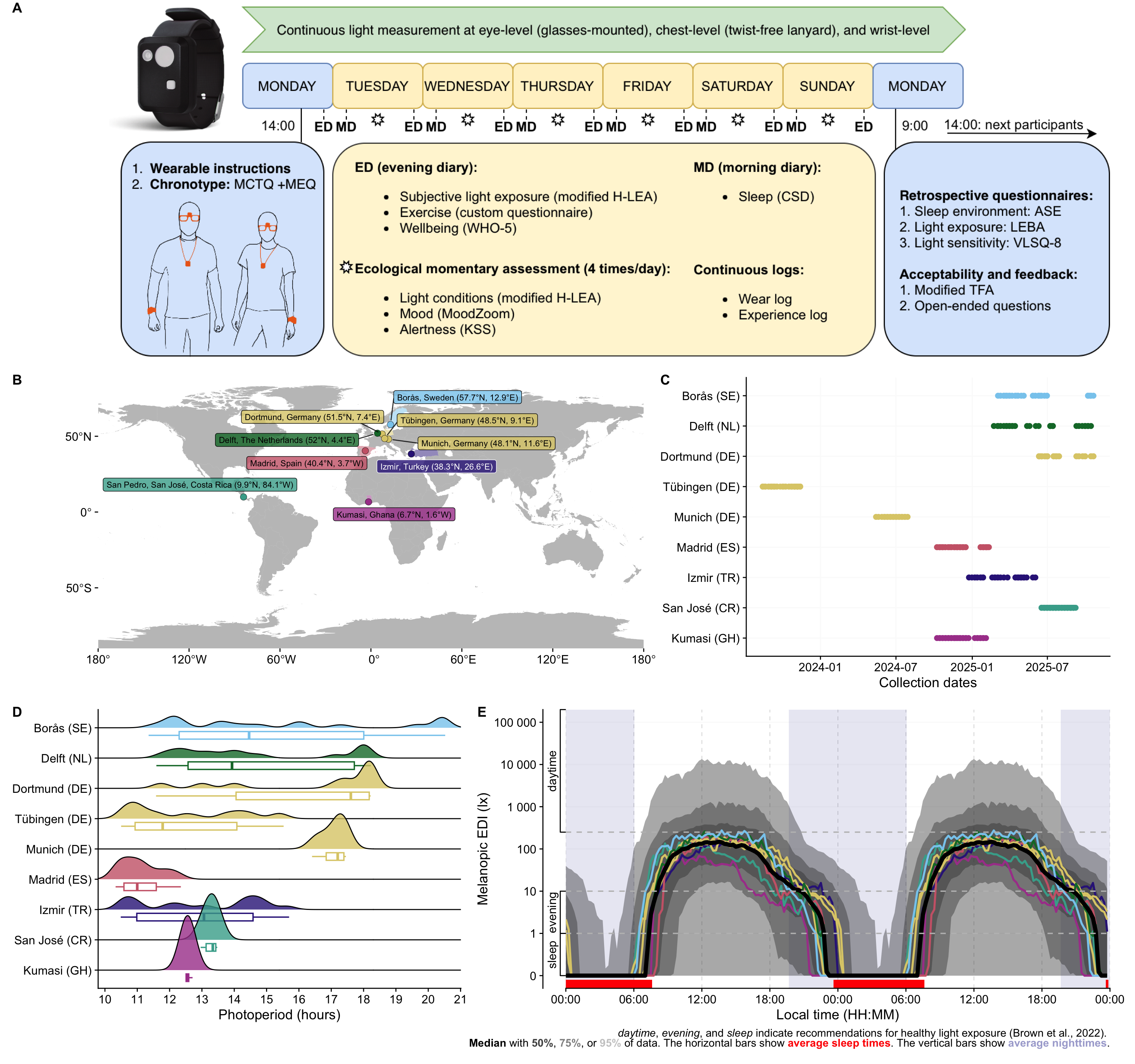
## Figure 1: Overview
### Panel A: Protocol
```{r}
path <- "assets/2026-03-30_MeLiDos_Protocol.png"
P_A <-
ggdraw() +
  draw_image(path)
P_A
```
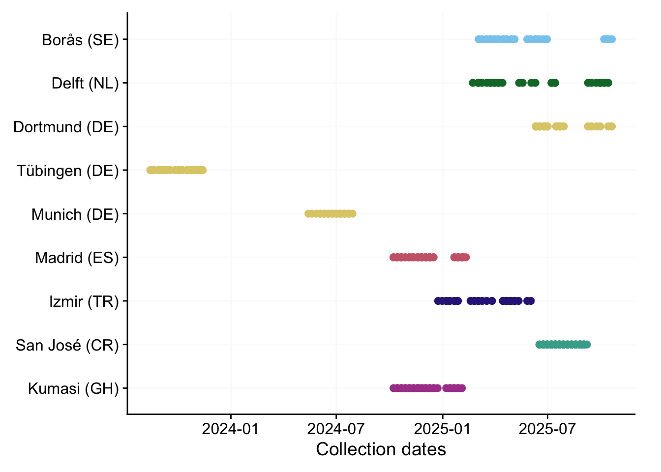
### Panel B: Overview
```{r}
P_B <-
  light_glasses_processed2 |>
  rbind(light_chest_processed2) |>
  distinct(site, Id, Datetime) |>
  mutate(site = fct(site, levels = names(melidos_cities))) |>
  site_conv_mutate() |>
  gg_overview(Id.colname = site, gap.data = tibble(),
              color = site) +
  scale_color_manual(values = melidos_colors) +
  guides(color = "none") +
  labs(y = NULL, x = "Collection dates")
P_B
```
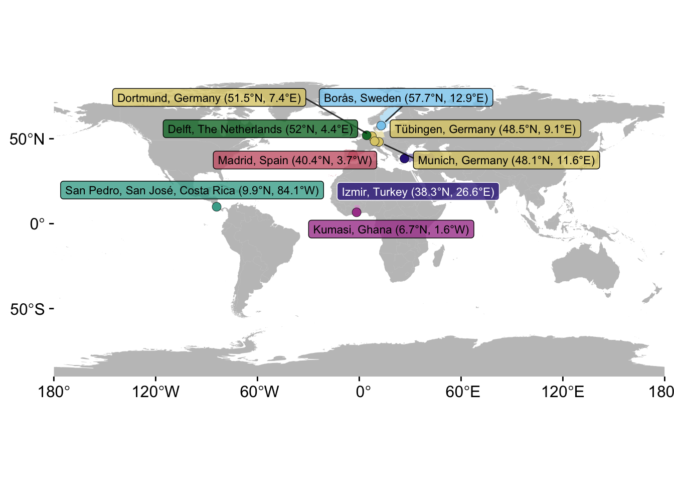
### Panel C: Location
```{r}
world <- ne_countries(scale = "medium", returnclass = "sf")

    countries_colors <- tibble(
      country = melidos_countries,
      color   = melidos_colors,
      stringsAsFactors = FALSE
    )

    world$color <- ifelse(
      world$name %in% countries_colors$country,
      countries_colors$country[match(world$name, countries_colors$country)],
      NA
    )

    # 3) Locations in geographic CRS (EPSG:4326)
    location_info <- tibble(
      country  = melidos_countries,
      location = melidos_cities,
      lat      = melidos_coordinates |> map(1) |> unlist(),
      lon      = melidos_coordinates |> map(2) |> unlist(),
      color    = melidos_countries,
      stringsAsFactors = FALSE
    ) |>
      rowwise() |>
      mutate(
        coordinate_string = format_coordinates(c(lat,lon)),
        label =
          paste0(location, ", ", country, " (", coordinate_string, ")")
        )

    locations <- st_as_sf(location_info, coords = c("lon", "lat"), crs = 4326)

    # 4) Project both layers to a planar CRS
    # robinson_crs <- paste0("+proj=", map_projection)
    robinson_crs <- "+proj=eqc"
    world_proj     <- st_transform(world,    crs = robinson_crs)
    locations_proj <- st_transform(locations, crs = robinson_crs)

    bb <- st_bbox(world_proj)
    y_offset <- 0.08 * (bb["ymax"] - bb["ymin"])

    # 5) Plot
P_C <-
      ggplot() +
      geom_sf(data = world_proj, aes(fill = color),
              color = NA, size = 0.25, alpha = 0.5, show.legend = FALSE) +
      geom_sf(data = locations_proj, aes(fill = color),
              shape = 21, color = "black", size = 3, stroke = 0.2) +
      geom_label_repel(
        data = locations_proj,
        stat = "sf_coordinates",
        label.size = 0,
        aes(label = label, fill = color, geometry = geometry),
        color = c(rep("black", 8), "white"),
        min.segment.length = 0.75,
        size = 3,
        alpha = 0.8,
        box.padding = 0.35,    # space between labels
        max.overlaps = 20,
        point.padding = 0.25,  # space from point to label
        force = 2.5,             # stronger repulsion
        force_pull = 0.25,      # weaker pull back to point
        seed = 123
      ) +
      scale_fill_manual(values =
                          countries_colors |>
                          select(country, color) |>
                          deframe()) +
      theme_cowplot() +
      theme(legend.position = "none") +
      theme_sub_axis(line = element_blank()) +
      labs(x = NULL, y = NULL) +
      coord_sf(expand = FALSE)
P_C
```
### Panel D: Doubleplot
```{r}
source("scripts/Brown_bracket.R")
```
```{r}
P_D_data <-
      light_glasses_processed2 |>
      ungroup() |>
      mutate(across(where(is.POSIXct),
                    \(x) {
                      date(x) <- "2025-04-03"
                      x }),
             across(c(dawn, dusk),
                    LightLogR:::datetime_to_circular)
             ) |>
      aggregate_Datetime(
        unit = "15 mins",
        type = "floor",
        numeric.handler = \(x) median(x, na.rm = TRUE),
        upper95 = quantile(MEDI, 0.975, na.rm = TRUE),
        upper75 = quantile(MEDI, 0.875, na.rm = TRUE),
        upper50 = quantile(MEDI, 0.75, na.rm = TRUE),
        lower50 = quantile(MEDI, 0.25, na.rm = TRUE),
        lower75 = quantile(MEDI, 0.125, na.rm = TRUE),
        lower95= quantile(MEDI, 0.025, na.rm = TRUE),
      ) |>
        mutate(
          across(c(dawn, dusk), LightLogR:::circular_to_hms),
          across(c(dawn, dusk),
                 \(x) {
                      x <- x |> strptime("%H:%M:%S", tz = tz(Datetime))
                      date(x) <- "2025-04-03"
                      x |> as.POSIXct() }),
               )

P_D_data_site <-
    light_glasses_processed2 |>
    ungroup(Id) |>
    select(site, Datetime, MEDI) |>
    aggregate_Date(
        unit = "15 mins",
        type = "floor",
        numeric.handler = \(x) {
          median(x, na.rm = TRUE)
          },
        date.handler = \(x) median(x, na.rm = TRUE),
        upper95 = quantile(MEDI, 0.975, na.rm = TRUE),
        upper75 = quantile(MEDI, 0.875, na.rm = TRUE),
        upper50 = quantile(MEDI, 0.75, na.rm = TRUE),
        lower50 = quantile(MEDI, 0.25, na.rm = TRUE),
        lower75 = quantile(MEDI, 0.125, na.rm = TRUE),
        lower95= quantile(MEDI, 0.025, na.rm = TRUE),
      ) |>
    mutate(
      across(where(is.POSIXct),
                    \(x) {
                      date(x) <- "2025-04-03"
                      x })
    )

P_D_data_site <-
  P_D_data_site |>
  rbind(
    P_D_data_site |>
    mutate(
      across(where(is.POSIXct),
                    \(x) {
                      date(x) <- "2025-04-04"
                      x })
    )
    )

# site_color <- ggsci::pal_jco()(1)
site_color <- "black"

P_D <-
P_D_data |>
      mutate(sleep = replace_values(sleep, "wake" ~ NA),
             ) |>
      gg_doubleplot(geom = "blank",
                    facetting = FALSE,
                    # jco_color = FALSE,
                    x.axis.label = "Local time (HH:MM)",
                    y.axis.label = "Melanopic EDI (lx)",
                    aes_fill = site
                    ) |>
      gg_photoperiod(fill = "darkblue", alpha = 0.1) |>
      gg_states(sleep, aes_fill = sleep, ymax = -0.1, fill = "red", alpha = 1,
                on.top = TRUE) +
      geom_ribbon(aes(ymin = lower95, ymax = upper95), alpha = 0.4) +
      geom_ribbon(aes(ymin = lower75, ymax = upper75), alpha = 0.4) +
      geom_ribbon(aes(ymin = lower50, ymax = upper50), alpha = 0.4) +
      geom_line(data = P_D_data_site |>       site_conv_mutate(),
                aes(y=MEDI, colour = site), linewidth = 1) +
      geom_line(aes(y = MEDI), linewidth = 2) +
      map(c(1,10,250),
          \(x) geom_hline(aes(yintercept = x), col = "grey", linetype = "dashed")
      ) +
      scale_color_manual(values = melidos_colors) +
      coord_cartesian(ylim = c(0, 100000)) +
      guides(y = guide_axis_stack(Brown_bracket, "axis"), fill = "none",
             color = "none") +
      # labs(x = NULL)
      labs(
        caption = glue(
          "<i>daytime</i>, <i>evening</i>, and <i>sleep</i> indicate
          recommendations for healthy light exposure (Brown et al., 2022).
          <br><b>Median</b> with <b style = 'color:{alpha(site_color,
          alpha = 0.75)}'>50%</b>, <b style = 'color:{alpha(site_color,
          alpha = 0.5)}'>75%</b>, or <b style = 'color:{alpha(site_color,
          alpha = 0.25)}'>95%</b> of data. The horizontal bars show
          <b style = 'color:red'>average sleep times</b>. The vertical bars show
          <b style = 'color:{alpha('darkblue', alpha = 0.4)}'>average nighttimes</b>."
        )
      ) +
      theme(plot.caption = ggtext::element_markdown())
P_D
```
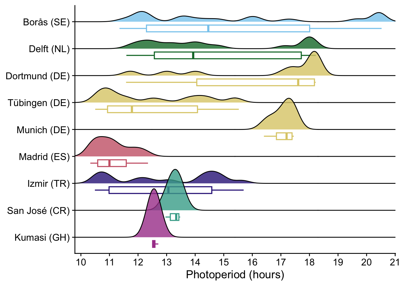
### Panel E: Photoperiods
```{r}
tz <- light_glasses_processed2 |> pull(Datetime) |> tz()

photoperiods <- metrics_chest$data[[3]] |> pull(photoperiod)

photoperiods_range <- photoperiods |> range() |> round(1)

photoperiods_seq <-
      inject(seq(!!!photoperiods_range, by = 1) |>
               round(1))

P_E_data <-
      metrics_glasses$data[[3]] |>
      rbind(metrics_chest$data[[3]]) |>
      distinct(site, Id, Date, .keep_all = TRUE) |>
      mutate(site = site |> fct_rev()) |>
      site_conv_mutate()

P_E <-
P_E_data |>
      ggplot(aes(x=photoperiod)) +
      geom_boxplot(aes(y= site, col = site), width = 0.25,
                   position = position_nudge(y = -0.25)) +
      geom_density_ridges(aes(y=site, fill = site),
                          bandwidth = 0.25,
                          alpha = 0.8) +
      scale_x_continuous(breaks = 10:21) +
      scale_color_manual(values = melidos_colors) +
      scale_fill_manual(values = melidos_colors) +
      labs(
        y = NULL,
        x = "Photoperiod (hours)"
        ) +
      theme_cowplot() +
      guides(
        fill = "none", color = "none") +
      coord_cartesian(xlim = photoperiods_range) +
      theme(axis.title.x = ggtext::element_markdown())
P_E
```
### Plot composition
```{r}
#| fig-height: 15
#| fig-width: 16
P_A /
  ((P_C + P_B) + plot_layout(widths = c(3,2))) /
  ((P_E + P_D) + plot_layout(widths = c(2,3))) +
  plot_layout(heights = c(1.3,1,1)) +
  plot_annotation(tag_levels = "A")
ggsave("figures/Fig1.pdf", height = 10, width = 10.5, scale = 1.5)
ggsave("figures/Fig1.png", height = 10, width = 10.5, scale = 1.5)
```
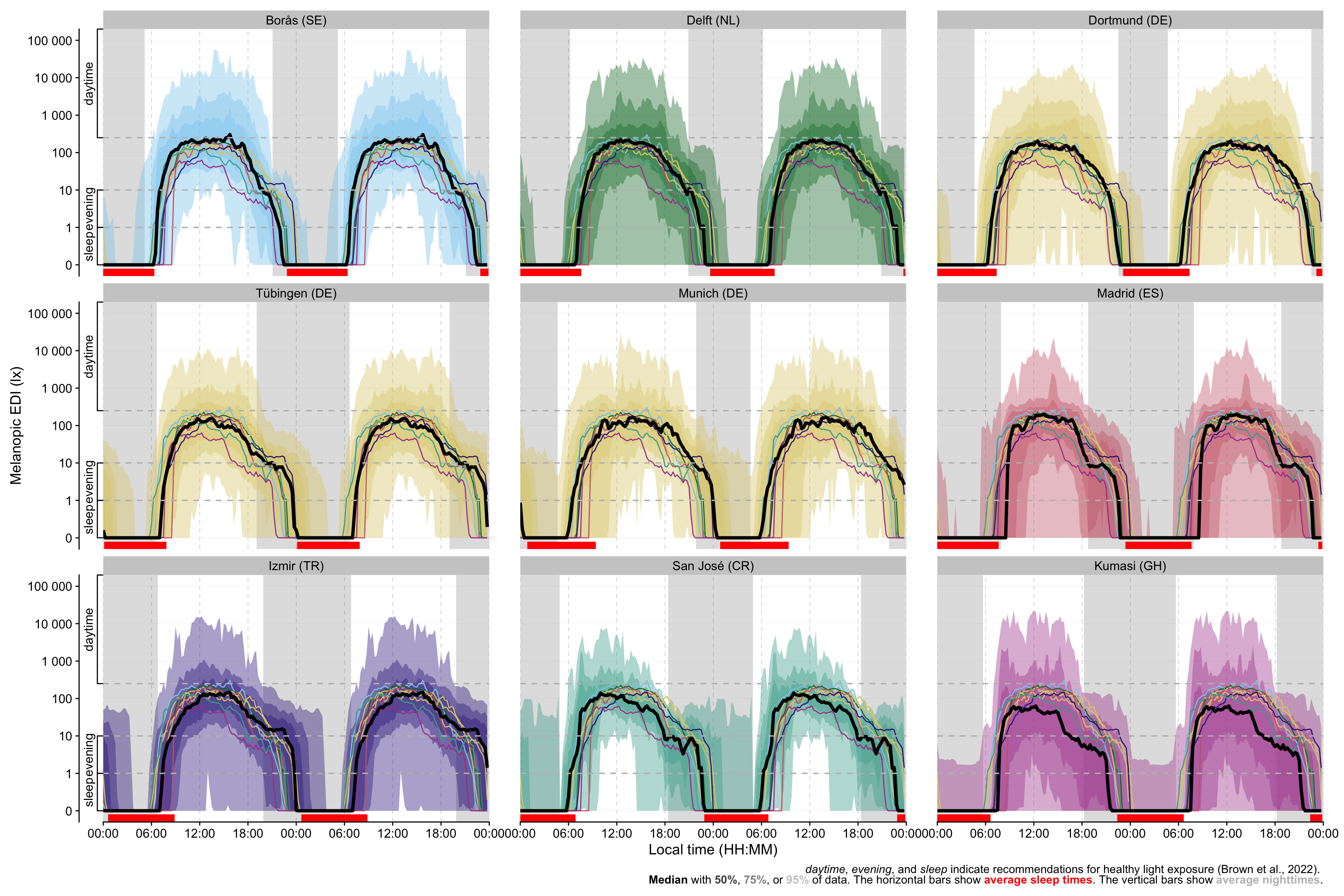
## Figure 2: Site plots
```{r}
Fig2_data <-
      light_glasses_processed2 |>
      ungroup(Id) |>
      mutate(across(where(is.POSIXct),
                    \(x) {
                      date(x) <- "2025-04-03"
                      x }),
             across(c(dawn, dusk),
                    LightLogR:::datetime_to_circular)
             ) |>
      aggregate_Datetime(
        unit = "15 mins",
        type = "floor",
        numeric.handler = \(x) median(x, na.rm = TRUE),
        upper95 = quantile(MEDI, 0.975, na.rm = TRUE),
        upper75 = quantile(MEDI, 0.875, na.rm = TRUE),
        upper50 = quantile(MEDI, 0.75, na.rm = TRUE),
        lower50 = quantile(MEDI, 0.25, na.rm = TRUE),
        lower75 = quantile(MEDI, 0.125, na.rm = TRUE),
        lower95= quantile(MEDI, 0.025, na.rm = TRUE),
      ) |>
        mutate(
          across(c(dawn, dusk), LightLogR:::circular_to_hms),
          across(c(dawn, dusk),
                 \(x) {
                      x <- x |> strptime("%H:%M:%S", tz = tz(Datetime))
                      date(x) <- "2025-04-03"
                      x |> as.POSIXct() }),
               )
```
```{r}
#| fig-width: 18
#| fig-height: 12
# Fig2 <-
Fig2_data |>
      mutate(sleep = replace_values(sleep, "wake" ~ NA),
             ) |>
      site_conv_mutate(rev = FALSE) |>
      gg_doubleplot(geom = "blank",
                    facetting = FALSE,
                    jco_color = FALSE,
                    x.axis.label = "Local time (HH:MM)",
                    y.axis.label = "Melanopic EDI (lx)",
                    aes_fill = site
                    ) |>
      gg_photoperiod() |>
      gg_states(sleep, aes_fill = sleep, ymax = -0.1, fill = "red", alpha = 1,
                on.top = TRUE) +
      facet_wrap(~site, nrow = 3, ncol = 3, dir = "lt") +
      geom_ribbon(aes(ymin = lower95, ymax = upper95, fill = site), alpha = 0.4) +
      geom_ribbon(aes(ymin = lower75, ymax = upper75, fill = site), alpha = 0.4) +
      geom_ribbon(aes(ymin = lower50, ymax = upper50, fill = site), alpha = 0.4) +
      geom_line(aes(y = MEDI, col = site), linewidth = 0.5, layout = "fixed") +
      geom_line(aes(y = MEDI), linewidth = 1.5) +
      map(c(1,10,250),
          \(x) geom_hline(aes(yintercept = x), col = "grey", linetype = "dashed")
      ) +
      scale_color_manual(values = melidos_colors) +
      scale_fill_manual(values = melidos_colors) +
      coord_cartesian(ylim = c(0, 100000)) +
      guides(y = guide_axis_stack(Brown_bracket, "axis"), fill = "none",
             color = "none") +
      # labs(x = NULL)
      labs(
        caption = glue(
          "<i>daytime</i>, <i>evening</i>, and <i>sleep</i> indicate
          recommendations for healthy light exposure (Brown et al., 2022).
          <br><b>Median</b> with <b style = 'color:{alpha(site_color,
          alpha = 0.75)}'>50%</b>, <b style = 'color:{alpha(site_color,
          alpha = 0.5)}'>75%</b>, or <b style = 'color:{alpha(site_color,
          alpha = 0.25)}'>95%</b> of data. The horizontal bars show
          <b style = 'color:red'>average sleep times</b>. The vertical bars show
          <b style = 'color:grey'>average nighttimes</b>."
        )
      ) +
      theme(plot.caption = ggtext::element_markdown(),
            panel.spacing.x = unit(30, "pt"))
ggsave("figures/Fig2.pdf", height = 8, width = 12, scale = 1.5)
ggsave("figures/Fig2.png", height = 8, width = 12, scale = 1.5)
```
```{r}
walk(names(melidos_cities),
     \(x) Fig2_data |>
            Fig2_plot_individual(x) |>
            ggsave(plot = _,
                   filename = str_c("figures/Fig2_individual/Fig2_",x ,".pdf"),
                   width = 8,
                   height = 5
                   )
     )
```
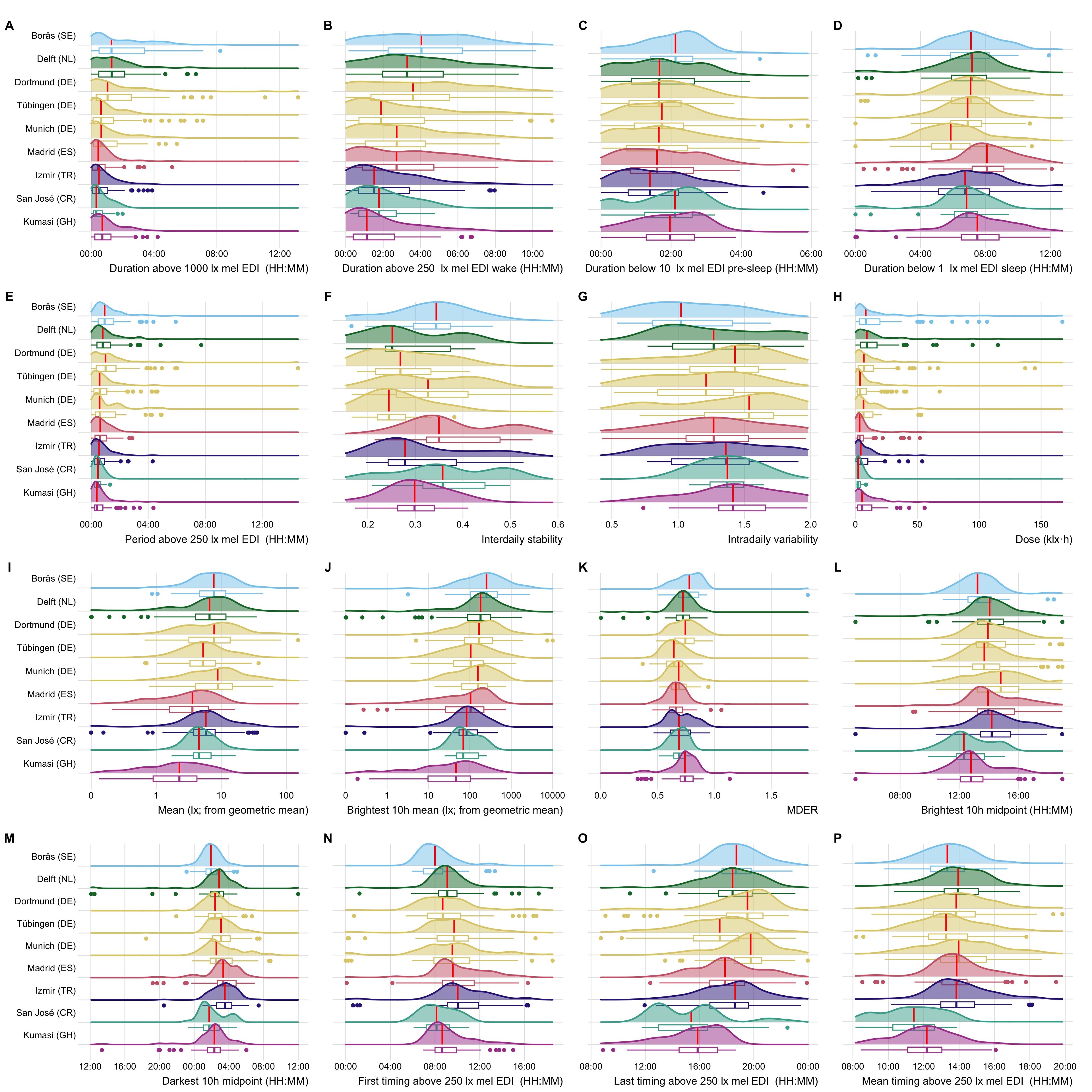
## Figure 3: Metric plots
```{r}
Fig3_data <-
tbl2_data |>
  mutate(name =
           name |>
           str_to_sentence() |>
           str_replace_all("_", " ") |>
           str_replace("(1000$|250 |250$|10 |1 )",
                       "\\1 lx mel EDI ") |>
           str_replace("Mder", "MDER"),
         name = name |>
           replace_when(
             metric_type == "duration" ~ str_c(name, " (HH:MM)"),
             metric_type == "level" ~ str_c(name, " (lx; from geometric mean)"),
             metric_type == "exposure history" ~ str_c(name, " (klx·h)"),
             metric_type == "timing" ~ str_c(name, " (HH:MM)")
           ),
         data = data |> map2(metric_type, \(x,y) {
           if(y %in% c("duration", "timing")) {
           x |> mutate(metric = metric*60*60)
         } else x
         })
         )

Fig3_data <-
  Fig3_data |>
  mutate(
    plot = pmap(list(data, scaling, metric_type, name), Fig3_plot)
  )
```
```{r}
#| fig-height: 20
#| fig-width: 20
#| message: false
#| warning: false
Fig3 <-
  Fig3_data |>
  filter_out(name == "Darkest 10h mean (lx; from geometric mean)") |>
  pull(plot) |>
  reduce(\(plots, plot) `+`(plots, plot))
Fig3 + plot_annotation(tag_levels = "A") &
  theme(
    plot.tag = element_text(face = "bold")
  )
ggsave("figures/Fig3.pdf", width = 10, height = 10, scale = 2)
ggsave("figures/Fig3.png", width = 10, height = 10, scale = 2)
```
```{r}
walk2(Fig3_data$plot,
      LETTERS[1:17],
      \(x,y) ggsave(str_c("figures/Fig3_individual/Fig3_",
                          y,
                          ".pdf"),
                    x+ theme_sub_axis_left(text = element_text()),
                    width = 3.5,
                    height = 5)
      )
```
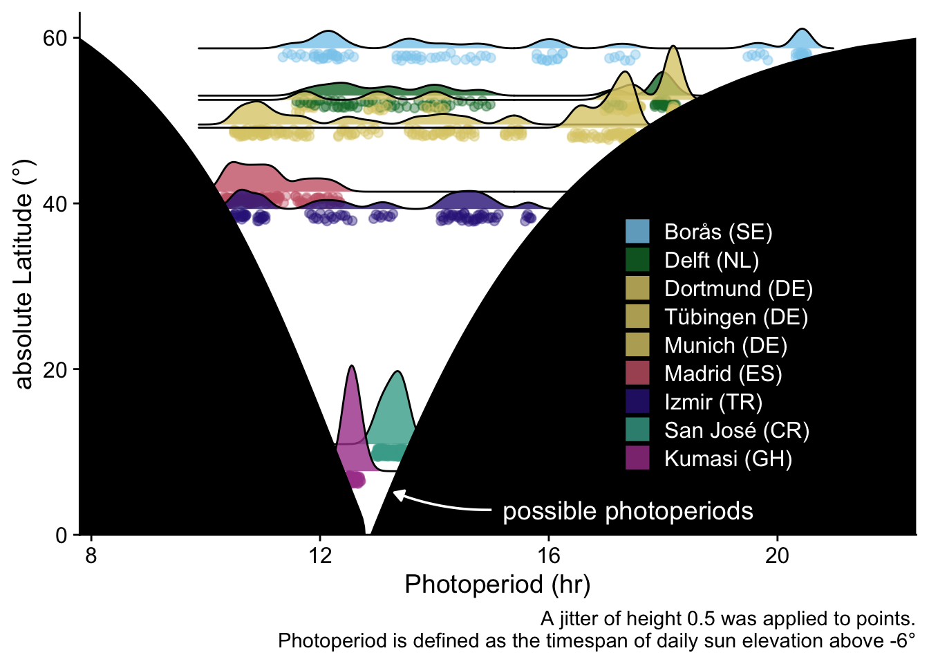
## Figure: latitude x photoperiod
```{r}
span_phot <- tibble(Datetime = as.POSIXct(ymd("2025-01-01"), tz = "UTC") + ddays(0:364))

phot_potential <-
0:60 |>
  map(
   \(x) span_phot |>
        extract_photoperiod(c(x,0)) |>
        group_by(lat) |>
        summarize(min = min(photoperiod),
                  max = max(photoperiod))
) |> list_rbind()

phot_potential_range <-
  phot_potential |> summarize(min = min(min), max = max(max)) |> unlist()

P_E_data |>
  mutate(site = fct_rev(site)) |>
  # site_conv_mutate(rev = TRUE) |>
  ggplot(aes(y = lat)) +
  geom_jitter(aes(col = site, x = photoperiod), width = 0, height = 0.5, alpha = 0.4) +
  geom_density_ridges(aes(y=lat, fill = site, x = photoperiod),
                      scale = 2,
                          position = position_nudge(y = 1),
                          bandwidth = 0.15,
                          alpha = 0.8) +
  geom_ribbon(data = phot_potential, aes(xmin = 0, xmax = min), fill = "black") +
  geom_ribbon(data = phot_potential, aes(xmin = max, xmax = 24), fill = "black") +
  annotate("text", y = 3, x = 15.2, label = "possible photoperiods", color = "white",
           hjust = 0) +
  annotate("curve", y = 3, x = 15,
           xend = 13.3, yend = 5.1,
           curvature = -0.1,
           arrow = arrow(type = "closed",
                         length = unit(0.2, "cm")),
           color = "white") +
  theme_cowplot() +
  guides(color = "none") +
  coord_cartesian(ylim = c(0, 63), expand = FALSE, xlim = phot_potential_range) +
  scale_color_manual(values = melidos_colors) +
  scale_fill_manual(values = melidos_colors) +
  labs(color = "Site", x = "Photoperiod (hr)", y = "absolute Latitude (°)",
       caption = "A jitter of height 0.5 was applied to points.\nPhotoperiod is defined as the timespan of daily sun elevation above -6°") +
  theme(
    # panel.background = element_rect(fill = "black"),
        legend.position = "inside",
        legend.text = element_text(colour = "white"),
        legend.position.inside = c(0.65,0.4))
ggsave("figures/photoperiod_potential_ridges.pdf", width = 6, height = 6)
ggsave("figures/photoperiod_potential_ridges.png", width = 6, height = 6)
```
## Table: Personal light exposure vs. recommendations
```{r}
Brown.by.site <-
light_glasses_processed2 |>
  Brown2reference(
    Brown.day = "wake",
    Brown.evening = "pre-sleep",
    Brown.night = "sleep"
  ) |>
  drop_na(Reference.check) |>
  group_by(site, State.Brown, Reference.check) |>
  durations() |>
  pivot_wider(names_from = Reference.check, names_prefix = "check_", values_from = duration) |>
  mutate(adhered = check_TRUE,
         duration = check_FALSE + check_TRUE,
         adherence = check_TRUE / duration)

Brown.by.site.total <-
Brown.by.site |>
  group_by(site) |>
  summarize(adhered = sum(adhered) |> as.duration(),
            duration = sum(duration) |> as.duration(),
            adherence = adhered/duration,
            State.Brown = "total")

Brown.by.site <-
Brown.by.site |>
  select(site, State.Brown, adhered, duration, adherence) |>
  bind_rows(Brown.by.site.total) |>
  pivot_wider(names_from = State.Brown, values_from = c(adhered, duration, adherence))

Brown_missing <-
  light_glasses_processed2 |>
  Brown2reference(
    Brown.day = "wake",
    Brown.evening = "pre-sleep",
    Brown.night = "sleep"
  ) |>
  group_by(site) |>
  durations(Reference.check, show.missing = TRUE) |>
  mutate(missing_pct = missing/total) |>
  select(site, missing_pct, missing, total)

Brown_overall <-
Brown.by.site |>
  left_join(Brown_missing, by = "site") |>
  ungroup() |>
  summarize(site = "Overall",
            adherence_wake = sum(adhered_wake)/sum(duration_wake),
            `adherence_pre-sleep` = sum(`adhered_pre-sleep`)/sum(`duration_pre-sleep`),
            adherence_sleep = sum(adhered_sleep)/sum(duration_sleep),
            adherence_total = sum(adhered_total)/sum(duration_total),
            fraction_wake = sum(duration_wake)/sum(total),
            `fraction_pre-sleep` = sum(`duration_pre-sleep`)/sum(total),
            fraction_sleep = sum(duration_sleep)/sum(total),
            fraction_missing = sum(missing)/sum(total))

Brown_summary <-
Brown.by.site |>
  left_join(Brown_missing, by = "site") |>
  mutate(
    fraction_wake = (duration_wake)/(total),
    `fraction_pre-sleep` = (`duration_pre-sleep`)/(total),
    fraction_sleep = (duration_sleep)/(total),
    fraction_missing = (missing)/(total)
  ) |>
  select(-starts_with("adhered_"), -starts_with("duration_"), -total, -missing_pct, -missing) |>
  site_conv_mutate(rev = FALSE) |>
  arrange(site)
```
```{r}
source("scripts/RQ2_specific.R")
Brown_table <-
bind_rows(Brown_overall, Brown_summary) |>
  gt() |>
  gt::rows_add(site = NA, .after = 1)|>
  tab_style(
    style = list(css(`padding-top` = "0px",
            `padding-bottom` = "0px"),
            cell_fill("lightgrey")
            ),
    locations = cells_body(rows = 2)) |>
  sub_missing(missing_text = "") |>
  fmt_percent(decimals = 0) |>
  tab_spanner("Adherence to recommendations during:", starts_with("adherence_")) |>
  tab_spanner("Percentage of measured time:", starts_with("fraction_")) |>
  cols_label_with(fn = \(x) str_remove(x, "adherence_|fraction_") |> str_to_sentence()) |>
  tab_style(
    style = cell_text(weight = "bold"),
    locations = list(
      cells_body(site),
      cells_column_labels(),
      cells_column_spanners(),
      cells_body(rows = 1)
    )
  ) |>
  gt_multiple(
    melidos_colors |> names(),
    style_rows
  ) |>
  tab_style(
    style = cell_borders("right", "lightgrey", weight = "2px"),
    locations = cells_body(adherence_total)
  ) |>
  tab_style(
    style = cell_text(align = "center"),
    list(cells_body(), cells_column_labels())
  ) |>
  tab_footnote(
    "Missingness can result from either missing sleep-wake diary data for a given day, and/or missing or removed measurements of melanopic EDI",
    cells_column_labels(fraction_missing)
  ) |>
  tab_footnote(
    "Recommendations for healthy lighting refer to Brown et al. (2022). Wake ≥ 250lx melanopic EDI, pre-sleep ≤ 10lx melanopic EDI, sleep ≤ 1lx melanopic EDI",
    cells_column_spanners(1)
  ) |>
  tab_footnote(
    "Total is a time-weighted average",
    cells_column_labels(adherence_total)
  )
```
```{r}
Brown_table
gtsave(Brown_table, "tables/Brown_table.png")
```
## Session Info
```{r}
sessionInfo()
```